Wilson Interval Interview Lab: Diagnose Rare-Event Coverage and Zero-Success Samples
Quick Overview
Calculate Wilson intervals for zero and rare successes, compare Wald and exact methods, and diagnose coverage by enumerating fixed-n binomial outcomes. Original worked cases, primary references and explicit verification boundaries support focused interview practice.
The Wilson interval avoids the collapsed zero-width estimate produced by the ordinary Wald interval when a binomial sample has no successes. Zero successes is an observation, not proof that the population probability is zero. Wilson gives a useful bounded interval, but its actual coverage still varies with sample size and the true rate—especially for rare events.
This original Wilson interval interview lab calculates boundary examples and enumerates repeated-sampling coverage exactly under a fixed-n binomial model. PracHub's statistics-screen practice supplies broader inference questions; this exercise focuses on what an interval procedure does when successes are scarce.
Official statsmodels, SciPy and NIST references establish interval methods and model context. The count table, coverage grid and interpretation exercises are original calculations. They are not observed conversion data, safety claims or a company's interview scoring rules. No candidate reports are being used as evidence.
State the binomial model before calculating uncertainty
Assume X follows a binomial distribution with fixed sample size n and common success probability p. Each observation is an independent Bernoulli trial under that probability. The data are the number of successes x, and the observed proportion is x/n. The interval procedure is evaluated under these assumptions, not independently of them.
For a product example, twenty rows are not necessarily twenty independent users. One person may generate several events, exposure probabilities may change over time, or the outcome definition may be misclassified. Changing the interval formula cannot repair a mismatch between the counting unit and the intended population inference.
The sample size is fixed in this lab. Repeatedly checking a dashboard and stopping when an interval looks favorable changes the procedure. So does selecting only a subgroup that produced an attractive result. The nominal confidence level belongs to a specified sampling and analysis rule, not to a decorative percentage printed beside any selected result.
Clarify whether the decision needs a two-sided interval or a one-sided upper bound. Our table uses two-sided 95% intervals throughout. A one-sided bound uses a different tail allocation and produces a different endpoint. Mixing a familiar rule-of-three approximation with a two-sided interval without stating the difference makes comparisons misleading.
Explain why the Wald interval collapses at zero
The usual Wald expression is p_hat ± z sqrt(p_hat(1-p_hat)/n). When x is zero, p_hat is zero and its plug-in standard error is also zero. The resulting interval is [0,0], even though a small positive population probability could easily have produced no successes in a small sample.
Clipping this interval to the valid probability range does not repair that collapse. It already lies inside the range. The problem is the uncertainty approximation at the boundary, not merely the possibility of an endpoint below zero or above one. A plot of valid-looking bounds can still conceal severe undercoverage.
For example, if the true rate is 0.001 and n is twenty, the probability of observing zero successes is approximately 98.0189%. The collapsed interval excludes that true positive probability whenever zero occurs. That one common outcome explains why a nominal 95% Wald procedure can have extremely poor coverage in this rare-event setting.
This is a statement about repeated samples generated under a hypothetical known rate. It does not assign a posterior probability to p after seeing zero. The frequentist coverage question asks how often the procedure includes a fixed true p across repetitions, not how likely p is to lie in one already computed interval.
Derive Wilson from the score inequality
Wilson comes from inverting the binomial score-test inequality, whose standard error is evaluated at the candidate population probability rather than replacing it immediately with the observed proportion. Solving the resulting quadratic yields a shifted center and a half-width with an additional boundary term.
from math import sqrt
from scipy.stats import norm

def wilson(x, n, alpha=0.05):
    z = norm.ppf(1-alpha/2)
    phat = x/n
    den = 1 + z*z/n
    center = (phat + z*z/(2*n))/den
    half = z*sqrt(phat*(1-phat)/n + z*z/(4*n*n))/den
    return max(0, center-half), min(1, center+half)
At zero successes, the mathematical lower bound is zero and the upper bound simplifies to z²/(n+z²). With twenty observations and z about 1.96, that upper bound is about 0.161125. The nonzero width preserves boundary uncertainty: the procedure has not interpreted an empty success count as infinite precision.
The statsmodels proportion interval reference provides Wilson and other methods. Our implementation is checked against its Wilson output on five count cases. Tiny floating-point lower endpoints near zero are displayed as zero; they are numerical artifacts, not evidence for a strictly positive lower probability after zero successes.
Do not present the shifted center as a newly observed success rate. The sample proportion remains x/n. The interval center is part of the construction used to quantify uncertainty. Confusing those quantities can make a report appear to claim that successes occurred when the actual count was zero.
Compare zero, rare and moderate counts
The original count table keeps the confidence convention fixed. Endpoints are proportions rather than percentages, and rounded values are shown only for readability. The complete results preserve higher precision. Wilson, Wald and Clopper–Pearson are calculated from the same x and n, so changes are attributable to the procedure rather than different data.
| Successes / trials | Observed rate | Wilson 95% interval | Wald 95% interval | Clopper–Pearson 95% interval |
|---|---|---|---|---|
| 0 / 20 | 0.00 | [0,0.1611] | [0,0] | [0,0.1684] |
| 0 / 100 | 0.00 | [0,0.0370] | [0,0] | [0,0.0362] |
| 1 / 20 | 0.05 | [0.0089,0.2361] | [0,0.1455] | [0.0013,0.2487] |
| 2 / 100 | 0.02 | [0.0055,0.0700] | [0,0.0474] | [0.0024,0.0704] |
| 50 / 100 | 0.50 | [0.4038,0.5962] | [0.4020,0.5980] | [0.3983,0.6017] |
Zero out of one hundred narrows the Wilson upper bound to about 3.6993%, compared with 16.1125% for zero out of twenty. Both samples observed no successes. The larger sample supplies more information, but neither result establishes a zero population rate or justifies a stronger claim than its model supports.
Notice that the exact interval is not uniformly wider at every endpoint: for zero out of one hundred, its upper endpoint is slightly lower than Wilson's. Coverage guarantees are properties of the entire procedure across possible counts. They do not imply a simple nesting relationship for every individual observed interval.
Near the center, Wilson and Wald look similar in the fifty-out-of-one-hundred case. That visual similarity does not validate Wald near the boundary. A useful interval comparison deliberately includes the count patterns that occur often under rare events, rather than testing only the most favorable moderate-rate example.
Enumerate coverage instead of estimating it by simulation
For fixed n and a hypothetical p, every possible success count is an integer from zero through n. Compute an interval for each count, mark whether it includes p, and sum the binomial probability masses of the included counts. This directly calculates finite-binomial coverage, subject only to numerical floating-point precision.
import numpy as np
from scipy.stats import binom
from statsmodels.stats.proportion import proportion_confint

counts = np.arange(n+1)
lo, hi = proportion_confint(counts, n, alpha=0.05, method='wilson')
covered = (lo <= p) & (p <= hi)
coverage = binom.pmf(counts, n, p)[covered].sum()
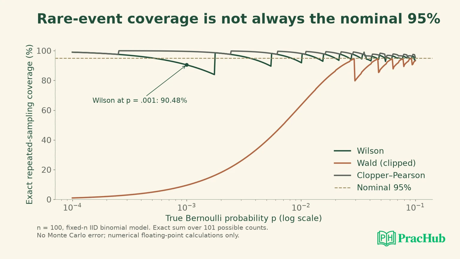
The lab evaluates n equal to twenty, one hundred and five hundred at rates 0.001, 0.01, 0.05 and 0.5. There is no Monte Carlo standard error because no repeated random draws are used for this grid. Adding a simulation-style uncertainty band would misdescribe how the reported coverage was obtained.
For n=20 and p=0.001, Wilson coverage is about 98.0189%, while Wald coverage is only 1.9811%. At p=0.05 with the same n, Wilson coverage is about 92.4516%, Wald 63.8940% and Clopper–Pearson 98.4098%. Wilson is dramatically better than Wald here, yet it does not attain at least 95% at every point.
For n=100 and p=0.001, Wilson coverage is approximately 90.4792%. This is a direct counterexample to the claim that “Wilson is a 95% interval, so coverage must always be 95%.” Discreteness produces changing inclusion patterns; nominal confidence and actual pointwise coverage are different quantities.
The SciPy binomial-test reference supplies related exact-binomial inference context, while the NIST reference discusses proportion interval construction. Our coverage values come from the explicit enumeration above, not from claiming that a library name alone establishes all inferential properties.
Choose an interval for the decision, not its reputation
Wilson is a useful default candidate because it handles boundaries far better than the ordinary plug-in Wald approximation. However, this lab intentionally displays an undercoverage case. If the application requires a conservative fixed-n binomial coverage guarantee, evaluate an exact construction and its costs rather than promising that Wilson provides that guarantee.
The central Clopper–Pearson construction can be conservative under the stated binomial model. Wider or uneven intervals affect decision usefulness, so compare both coverage and expected width. A method that includes the truth often but rarely supports a useful decision may not meet the same objective as a shorter approximate interval.
The procedure choice also depends on whether a threshold, a rate estimate or a comparison is required. A confidence interval for one proportion does not automatically supply a valid interval for a difference between two proportions. Comparing whether two individual intervals overlap is not a universal substitute for the intended two-sample procedure.
For a zero-success report, give the numerator and denominator alongside the interval and its method. “No successes in twenty independent fixed-n trials; two-sided Wilson 95% interval zero to about 16.1%” is inspectable. “The risk is zero” removes both the uncertainty and the assumptions that made the calculation meaningful.
Keep the executed boundary and the sampling boundary visible
Python 3.12.14, NumPy 2.5.3, SciPy 1.18.1 and statsmodels 0.15.0 produced the count cases and exact coverage grid. The custom Wilson implementation agrees with the library on the selected cases. The results are numerical checks of specified procedures, not empirical evidence about users or a live conversion funnel.
A production analysis still needs a defensible counting unit, exposure definition and observation window. Correlated events, missed successes, changing probabilities or outcome-dependent missingness can invalidate the binomial model. Neither an exact interval nor an improved approximation repairs that data-generating mismatch.
For an interview follow-up, alter one assumption at a time. Repeated events from each user suggest clustering; stopping after the first success suggests a different sampling design; a requirement for an upper risk limit suggests a one-sided procedure. Name the changed inference problem before selecting another formula.
For a concrete decision drill, declare a hypothetical threshold of 5percent before looking at the count. Zero out of 20 has a two-sided Wilson upper endpoint around16.1 percent, so that interval does not exclude rates above the threshold. Zero out of 100 has an upper endpoint around3.7 percent, so it fits below the threshold under this interval rule. The observed rate is zero in both cases; the uncertainty and resulting evidence differ. This is an interpretation of the saved count table, not an additional one-sided test or a guarantee outside the fixed-n model.
Rehearse uncertainty with the count attached
The following PracHub records develop proportion estimation, rare events and confidence intervals. They are related practice, not a dedicated Wilson test bank or a forecast of an employer's questions. Use the named task in the second column to keep the preparation focused.
| PracHub question | What to explain |
|---|---|
| Estimate Population Mean and Conversion Rate Accurately | Define the population and distinguish a rate estimate from its uncertainty. |
| Test Billboard Campaign Conversion Rate Exceeds 60% | Choose a one-sided test only when the decision calls for it. |
| Choose tests for rare-event A/B analysis | Diagnose sparse counts before using a normal approximation. |
| Derive variance and CTR confidence intervals | Derive the variance under the actual counting assumptions. |
| Design Sampling Strategy to Estimate Fake News Proportion | State the sampling unit and selection process before calculating bounds. |
Use the proportion-estimation question to compare zero out of twenty with zero out of one hundred. Then show the n=100, p=0.001 coverage counterexample. A defensible answer can recommend Wilson's boundary behavior while clearly stating what its nominal 95% label does not guarantee.
Sources and Further Reading
- statsmodels: Confidence intervals for a binomial proportion
- SciPy: Binomial test and proportion confidence intervals
- NIST: Confidence limits for a proportion
Sources checked November 3, 2026. Coverage is calculated by exact finite-binomial summation, not by a Monte Carlo experiment or an observed business dataset.
Comments (0)