XGBoost vs Random Forest: How ML Interviews Actually Probe the Difference
Quick Overview
A senior-level walkthrough of XGBoost vs random forest structured around the follow-up questions DS and MLE interviews actually ask: variance vs bias reduction, why boosting chases noisy labels, the tuning gap, parallelism, missing-value handling, calibration, and feature-importance pitfalls. Grounded in real interview questions from Amazon, TikTok, Capital One, Reddit, Point72, and OneMain Financial, ending with the judgment answer interviewers grade hardest.
Every DS and MLE loop has a version of this question, and most candidates answer it at the level of a library README: "XGBoost usually wins Kaggle, random forest is simpler." That answer fails the screen. The one that passes: random forest trains deep trees independently on bootstrap samples and averages them, which cuts variance. XGBoost trains shallow trees sequentially, each fitting the residual errors of the ensemble so far, which cuts bias, and it puts an explicit regularization penalty inside every split decision. Everything the interviewer asks next hangs off that one distinction, and this page walks the follow-ups in the order they actually come.
Key Takeaways
- Lead with the mechanism: bagging averages independent high-variance trees (variance reduction), boosting adds sequential low-bias corrections (bias reduction). Say "variance" and "bias" before anything else.
- Random forest is close to tuning-free: raise
n_estimatorsuntil the curve flattens, maybe touchmax_features. XGBoost's learning rate, depth, and subsampling interact, so quoting one "best value" for any of them is itself a red flag. - Noisy labels are the strongest case for the forest: boosting keeps re-fitting mislabeled points because their residuals never shrink, while bagging's averaging cancels independent mistakes.
- Neither model hands you calibrated probabilities once you reweight classes. If the downstream decision uses the probability (fraud cost thresholds, bid pricing), check a reliability curve and fit isotonic or Platt scaling on a holdout.
- The judgment answer interviewers want: ship the random forest baseline first, then move to XGBoost only if the measured validation gap pays for the tuning and monitoring it adds.
The first-screen answer: bagging cuts variance, boosting cuts bias
Asked in a Data Scientist interview — Compare trees, RF, and gradient boosting The candidate must compare decision trees, random forests, and gradient-boosted trees for supervised learning, list the key hyperparameters of each (from
max_featuresandbootstrapon the forest side tolearning_rateandsubsampleon the boosting side), and reason about the whole comparison through bias–variance and a sound validation plan.
A single deep decision tree is a low-bias, high-variance estimator. It can carve the training set almost perfectly, and a slightly different sample produces a very different tree. The two ensembles attack that from opposite ends.
Random forest draws B bootstrap samples, grows a deep, often depth-unlimited tree on each, and at every split considers only a random subset of features (max_features, √p by default for classification in scikit-learn). That last part is the one candidates forget. Predictions are averaged (regression) or majority-voted (classification). The math that makes this worth saying out loud: if each tree has variance σ² and the trees have pairwise correlation ρ, the variance of their average is
ρσ² + (1 − ρ)σ²/B
The second term dies as B grows, so the variance floor is ρσ². That is why the per-split feature subsampling exists: bootstrapping alone leaves trees highly correlated (they all find the same dominant splits), and lowering ρ is the only remaining lever. Bias stays roughly at the single-deep-tree level. More trees never overfit; they just cost more.
XGBoost builds an additive model. Tree k is fit not to the labels but to the gradients (and second derivatives) of the loss with respect to the current ensemble's predictions — the residuals, in the squared-error case. Each new tree is shallow (default max_depth=6), its contribution is shrunk by the learning rate η (default 0.3, and almost nobody ships the default), and the ensemble's bias falls with every round. Variance, meanwhile, accumulates: every tree is fit to errors the previous trees left, so the rounds are correlated by construction, and there is a point past which more rounds hurt. That is why XGBoost ships early stopping and random forest doesn't need it.
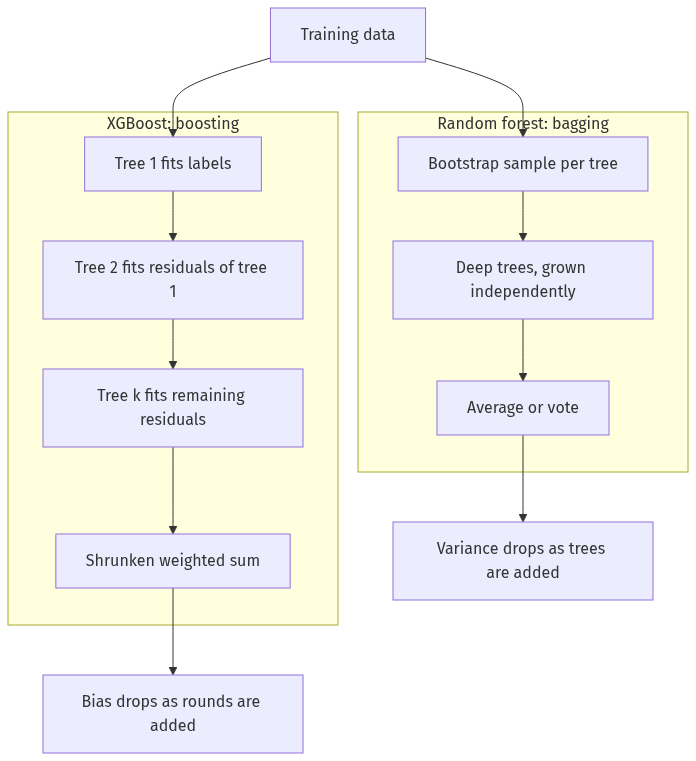
The common mistake at this stage is describing boosting as "trees that fix each other's mistakes" without saying sequentially on residuals with shrinkage. The phrase "fits the gradient of the loss" is what separates a candidate who used the library from one who read how it works. For a broader sweep of the surrounding theory, see the ML Knowledge Collection V2.
Here is the head-to-head most interviews eventually draw on the whiteboard:
| Dimension | Random forest | XGBoost |
|---|---|---|
| Tree depth | Deep, often unpruned | Shallow (depth 3–8 typical) |
| Trees trained | Independently, in parallel | Sequentially, on residuals |
| Error attacked | Variance | Bias |
| Overfitting from more trees | No (performance plateaus) | Yes (needs early stopping) |
| Regularization | Implicit (bagging + feature subsampling) | Explicit (λ, α, γ, η, subsampling) |
| Tuning burden | Low: n_estimators, max_features | High: η, depth, subsample, regularizers interact |
| Missing values | Imputation historically required | Learned default directions, native |
| Noisy labels | Averaging absorbs them | Residuals amplify them |
| Typical tabular accuracy | Strong baseline | Usually a bit better, if tuned |
Why boosting overfits noisy labels where bagging shrugs
Asked at TikTok — Explain and tune XGBoost; prevent overfitting The setup is a bad-seller classifier with roughly 0.5% positives. The candidate has to state XGBoost's actual training objective, show how the second-order Taylor expansion produces the split-gain formula, and explain what λ, α, γ, and the learning rate each do to bias and variance during split selection and pruning.
This TikTok question is the deepest common probe, and it is worth having the two formulas cold. XGBoost's objective for each new tree is the loss's second-order Taylor expansion plus a complexity penalty. Writing G and H for the sums of first and second derivatives of the loss over the instances in a leaf, the optimal leaf weight is
w* = −G / (H + λ)
and the gain from splitting a node into left and right is
gain = ½ [ G_L²/(H_L+λ) + G_R²/(H_R+λ) − (G_L+G_R)²/(H_L+H_R+λ) ] − γ
Read the knobs straight out of the formula. λ sits in the denominator, shrinking every leaf weight toward zero (L2 on the leaf values). γ is a fixed toll charged per split: if the gain doesn't clear it, the split doesn't happen, which is pruning stated as arithmetic. α (L1) pushes small leaf weights to exactly zero. η multiplies each tree's output before it joins the ensemble, so smaller η means each round corrects less and you need more rounds. That trade is the tuning problem, covered below.
Now the noisy-label story, because it is the sharpest practical difference between the two models. Suppose 3% of your labels are simply wrong: a fraud analyst mis-tagged the case, a delayed chargeback never arrived. In a random forest, each tree sees a bootstrap sample and fits some of that noise, but the mistakes are independent across trees and the average washes them out. In boosting, a mislabeled point is one the ensemble keeps getting "wrong," so its residual never shrinks. Round after round, trees allocate splits to chase it. With enough rounds the model memorizes the noise, and the damage is concentrated exactly where labels are least reliable.
The mitigations are the regularizers above plus subsample and colsample_bytree (each round sees a random fraction of rows and columns, which re-introduces a bit of bagging's independence) and, bluntly, early stopping on a clean validation set. But the interview-grade observation is this: if you know the labels are noisy — human-labeled data, weak supervision, delayed outcomes — that is a genuine argument for the forest, not just a smaller learning rate.
The tuning gap: the forest is nearly free, XGBoost is a coupled system
Asked at OneMain Financial — Select and tune XGBoost hyperparameters One million rows, 100 features (80 of them one-hot), a 1% positive rate, a single 16-core box with 32 GB of RAM, and a hard five-minute training budget. The candidate must pick hyperparameters that fit the budget, handle the imbalance, and set up validation grouped by user to avoid leakage.
Random forest tuning, in full: set n_estimators to a few hundred (error improves monotonically and flattens; there is no overfitting cliff to find), consider max_features, maybe floor the leaf size with min_samples_leaf on small data. The out-of-bag estimate gives you validation almost for free. This is why RF is the right first model: a trustworthy baseline costs almost nothing to stand up.
XGBoost is a different kind of object because its main knobs are coupled:
- η and
n_estimatorstrade against each other. Halve the learning rate and you need roughly twice the rounds to reach the same training loss. The sane pattern is to fix η around 0.05–0.1, set the round count high, and let early stopping choose the effective number. max_depthandmin_child_weightfight over interaction order. Depth 6 trees can express 6-way feature interactions;min_child_weight(a floor on H per leaf) vetoes leaves supported by too little effective data. Under a 1% positive rate this matters more than people expect: for logistic loss, H per instance is p(1−p), so confident predictions contribute almost nothing, and a moderatemin_child_weightquietly forbids splits isolating small pockets of positives.subsampleandcolsample_bytreeinteract with the two pairs above, so tune them after η and depth are pinned down rather than grid-searching everything jointly.
Under the OneMain constraints, the answer shape that passes: tree_method="hist" (the default since XGBoost 2.0, and the right call here — histogram split finding is what makes 1M×100 comfortable inside a minutes-scale CPU budget), depth 5–6, η≈0.1 with early stopping on a user-grouped validation split, and a decision, stated out loud, about scale_pos_weight. Reweighting positives helps ranking metrics but wrecks probability calibration, which is the next section's subject.
The mistake to avoid here is reciting a grid search. A grid over five coupled parameters at this scale blows the time budget by itself; the senior answer names which knobs matter, in what order, and what each one is for. For more ML tuning and theory prep, the MLE Knowledge Collection is a good next stop.
Training cost and parallelism: both parallelize, in different places
Asked at Amazon — Explain XGBoost Parallelism Strategies An entire question devoted to one topic: the candidate must explain how XGBoost exploits parallel hardware, first inside a single machine and then across a cluster, and reason about what those design choices cost in memory, speed, accuracy, and reproducibility.
"Random forest is parallel, XGBoost is sequential" is the folk answer, and it is half right in a way that fails this Amazon question. The correct picture has two levels.
Across trees, the forest is embarrassingly parallel: every tree is independent, so training parallelizes across cores with near-linear speedup (n_jobs=-1 and done). XGBoost is strictly sequential across boosting rounds: tree k needs the residuals left by trees 1..k−1, and no amount of hardware changes that.
Within a tree, the situation flips, and it helps to keep XGBoost's two designs distinct because candidates tend to blur them. The original exact method presorts each feature into a compressed column-block (CSC) layout so split scans run sequentially over memory. The newer hist method instead quantizes each feature into roughly 256 bins and accumulates gradient statistics (G and H) per bin, with per-feature histogram builds partitioned across threads. Across machines, workers hold row shards, build local histograms, and merge them with all-reduce at each tree level; that merge is where the synchronization cost and the mild non-determinism (floating-point reduction order) live. Binning is an approximation of exact greedy splitting, but the accuracy cost is negligible in practice, which is why hist became the default.
Be precise about the complexity, because this interview probes exactly that. Histograms do not make the O(rows × features) work disappear: exact greedy after its one-time presort scans O(rows × features) per tree level (each row lives in exactly one node per level), and histogram construction also touches every row for every feature once per level. The real speedup is structural: sequential, cache-friendly accumulation into bins instead of scattered scans over sorted values, the sibling-subtraction trick (build the smaller child's histogram, get the larger by subtracting from the parent's), and enumerating candidate splits over ~256 bins instead of every distinct feature value. In hist mode, memory is dominated by the quantized copy of the data rather than the trees. If the interviewer pushes to "what if the data doesn't fit on one machine," the answer is data-parallel sharding with all-reduce on histograms, not model parallelism, which cannot fit the algorithm's sequential outer loop.
Inference cost inverts the training story, and it is worth raising unprompted: a 500-tree unpruned forest is a large object with a long per-row walk, while a few hundred depth-6 boosted trees are compact and fast to evaluate. For latency-bound serving, XGBoost often wins even where accuracy ties. If you are prepping an Amazon loop specifically, start with the Amazon Machine Learning Engineer Interview Guide.
The follow-up probes: missing values, calibration, feature importance
A strong first answer buys you three follow-ups. These are where offers are separated from rejections, because each one has a folk answer that is subtly wrong.
Missing values: learned default directions vs imputation
Asked at Point72 — Explain and tune decision trees robustly A CART-focused grilling from a take-home follow-up: exact impurity formulas (Gini, entropy, variance), the split-selection rule, a defensible cross-validation plan for the tree hyperparameters, and how surrogate splits let a tree route rows whose split feature is missing.
XGBoost's handling is the one to explain precisely, because "it handles missing values" is the folk answer and the mechanism is the real one. During split finding, rows with a missing value for the candidate feature are tried down the left branch, then down the right; whichever direction yields more gain becomes that split's default direction, stored in the model. At inference, missing goes with the default. The elegant part: "missingness" gets treated as signal — if missing-income rows behave like high-risk rows, the model learns to route them that way, with no imputation step to maintain in the serving path.
One named gotcha: with scipy sparse input, XGBoost treats non-stored (implicit) entries as missing, while explicitly stored values, including an explicitly stored 0.0, are treated as real values (the missing parameter defaults to NaN). One-hot matrices behave the way people expect only because their zeros are typically not stored. Arithmetic on a CSR matrix can leave explicit zeros behind, and those entries are then values rather than missing, so two matrices that print identically can route rows differently.
Classic CART (the Point72 question) used surrogate splits instead: at each node, keep backup features whose splits mimic the primary one, and route missing rows by the best surrogate. Random forest implementations mostly dropped surrogates for speed, which is why the practical guidance for years was "impute before training a forest" — median/mode plus a missingness indicator column being the honest default. Recent scikit-learn releases added native missing-value support to trees and then to random forests, so hedge any "RF can't handle NaN" claim by implementation and version rather than stating it as a law of nature.
Calibration: the probabilities are not what they look like
Asked at Reddit — Build and evaluate click prediction models Given tabular click data with a roughly balanced label, the candidate must set a trivial baseline, then train and compare logistic regression, random forest, and gradient-boosted trees, with the stated goal being well-calibrated click probabilities for downstream ranking and decisioning, not just AUC.
Random forest probabilities are averages of per-tree votes, and an average of many imperfectly correlated trees almost never lands near 0 or 1. The classic empirical finding (Niculescu-Mizil and Caruana's model-calibration study) is that forests compress predictions away from the extremes: events the model should call near-certain come out scored as merely likely. AUC doesn't care, because ranking is preserved. Anything that thresholds on cost or multiplies the probability by a dollar value cares a great deal.
XGBoost with logistic loss is optimizing a proper scoring rule, so trained to convergence on enough data it comes out roughly calibrated — until you touch scale_pos_weight, which inflates every predicted probability by design, or stop very early, or regularize hard. The interview-grade answer to the Reddit question: compare models on log loss and a reliability diagram, not AUC alone; if the probabilities are consumed downstream, fit isotonic regression (or Platt scaling for small validation sets) on a held-out fold, and re-check after any reweighting. Logistic regression, for all its bias, is often the best-calibrated of the three out of the box, which is exactly why the question includes it.
Feature importance: the default numbers mislead in both models
Asked at Point72 — How would you explain PCA and SHAP? The candidate walks one real project end-to-end and must defend the interpretability choices: what PCA is doing to the feature space, and how SHAP attributes a tree model's predictions, with the interviewer probing whether they understand the tools or just imported them.
Impurity-based importance — feature_importances_ in both libraries' default — has two biases worth naming unprompted. It favors high-cardinality and continuous features because they simply offer more candidate split points, so an ID-like column can top the chart while carrying no generalizable signal. And it is computed on training data, so features that enabled overfitting look important precisely because they overfit.
The fixes, in the order to reach for them: permutation importance on a held-out set (shuffle one column, measure the metric drop — slow but honest), then SHAP via TreeExplainer when you need per-prediction attribution or directionality. Neither fully escapes correlated features: permutation creates impossible feature combinations when correlated columns are shuffled independently, and SHAP spreads credit across correlated features in ways that surprise stakeholders. Saying that limitation out loud is the senior signal; the follow-up trap in this Point72 question is the candidate who presents SHAP as ground truth.
"Which would you ship?" — the judgment answer
Asked at Capital One — Design a robust fraud detection system A fraud-detection design with hard numbers attached: a 0.2% fraud base rate, labels arriving on a 14-day delay via chargebacks, a p95 inference budget of 50 ms at 2,000 TPS, and an explicit cost matrix ($5 per false positive, $200 per false negative). Model choice has to be defended against all four constraints at once, starting with leakage-safe time-based splits.
This is where the comparison stops being academic, because every constraint in the Capital One prompt pushes on a different edge of the trade-off. Delayed, chargeback-derived labels mean label noise, an argument for bagging's tolerance or for conservative boosting with strong regularization and early stopping on a time-based split. The cost matrix means the probability is the product, so calibration on a recent holdout is mandatory before any threshold is set. The latency budget favors compact boosted trees at serving time. And a 0.2% base rate makes the scale_pos_weight-versus-calibration tension unavoidable rather than theoretical.
The shape of the answer that gets hired, at Capital One or anywhere this question appears:
- Baseline with a random forest (or even logistic regression) on day one. Nearly tuning-free, hard to misconfigure, and it establishes what "good" costs.
- Measure the gap. Tune XGBoost properly — hist method, early stopping, leakage-safe validation — and quantify the improvement in the metric that matters, here expected dollar loss, not AUC.
- Ship the upgrade only if the gap pays for what XGBoost adds: a tuning process someone must re-run when data drifts, early-stopping infrastructure, and a model more sensitive to label noise in exactly the freshest, least-settled labels.
- Say when you'd stay with the forest: small datasets, noisy labels, a team without tuning bandwidth, or a gap within the validation noise floor.
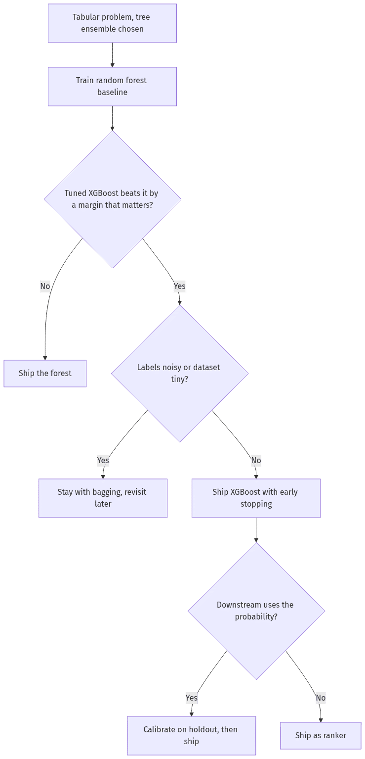
Notice what this answer is not: it is not "XGBoost, because it wins benchmarks." Interviewers ask "which would you ship" precisely to see whether you treat model choice as an engineering decision with costs on both sides. For a candidate's-eye account of preparing for these judgment-style ML interviews, see My MLE Interview Prep Journey: What Actually Worked.
Practice these on PracHub
Work these in roughly this order — each drills one layer of the comparison.
- Compare trees, RF, and gradient boosting — the comparison in its purest screen form: mechanisms, key hyperparameters of each, and the bias–variance framing.
- Explain and tune XGBoost; prevent overfitting (TikTok) — drills the objective, the gain formula, and what each regularizer does; the deepest theory probe on this page.
- Select and tune XGBoost hyperparameters (OneMain Financial) — tuning under a real compute budget with class imbalance and grouped validation.
- Explain XGBoost Parallelism Strategies (Amazon) — the systems layer: histogram split finding, block layout, distributed all-reduce.
- Explain key ML theory and techniques (Amazon) — a breadth question that mixes XGBoost parallelism with deep-learning topics like layer normalization; good pacing practice for a full onsite.
- Build and evaluate click prediction models (Reddit) — head-to-head model comparison where calibration, not AUC, is the graded output.
- Design a robust fraud detection system (Capital One) — the full judgment question: noisy delayed labels, cost matrices, and latency budgets forcing a defensible model choice.
- Build ETA prediction and simulate impact (DoorDash) — a regression take-home where a tree-ensemble baseline and its error analysis carry the exercise.
The full question bank filters by company and category if you want more ML questions from a specific loop, and the resources hub collects the longer prep guides referenced above.
Comments (0)