Google Machine Learning Engineer Interview Prep Guide

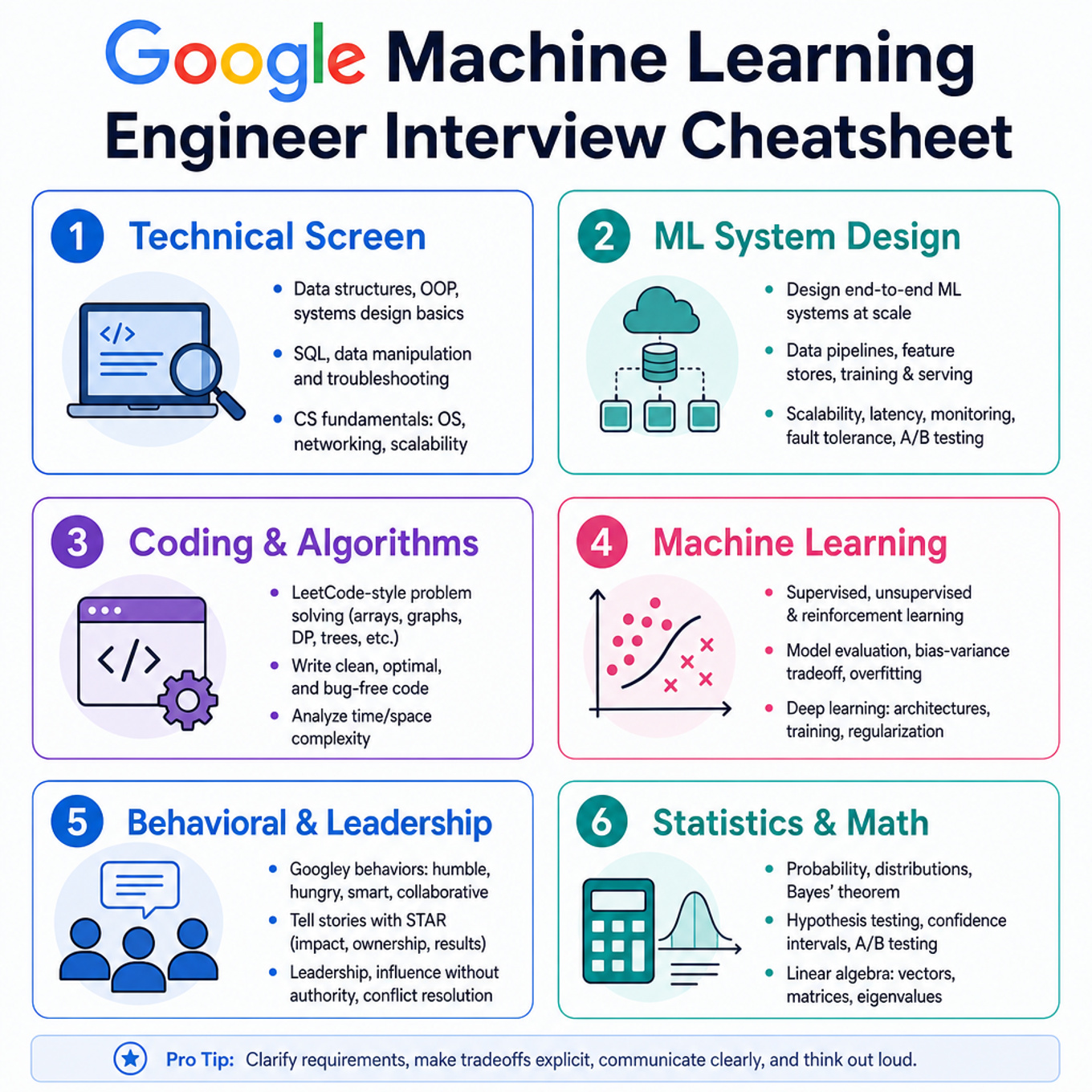
Focus most on Google-scale ML system design: recommendation/ranking, production serving, monitoring, and responsible AI, because your ML system design self-rating is 3/5 with only light system-design engagement so far. There are no clear strong areas from solved-question signals; coding has the most viewing activity, so graphs stay at normal review rather than being treated as mastered. The Google-specific emphasis is on Search/YouTube/Ads-style ranking, low-latency production ML, and fairness/privacy/safety expectations for high-impact models. Because your timeline is still exploratory, this is a breadth-first first pass of about 83 minutes before moving into timed practice and mock interviews.

Technical Screen — 42 min

ML System Design

• Recommendation Systems And Ranking (Focus) — covered in depth under Onsite below.

• Production ML Serving, Feature Stores, And Monitoring (Focus) — covered in depth under Onsite below.

• Responsible AI, Fairness, Privacy, And Safety In Google ML (Focus) — covered in depth under Onsite below.

This is relevant for Google-scale ML performance; review bottlenecks and communication trade-offs at medium depth.

What's being tested

Candidates must show practical mastery of distributing dense linear algebra across multiple accelerators: partitioning matrices, minimizing inter-GPU communication, and overlapping compute with transfers. Interviewers probe the candidate’s ability to trade compute vs communication, pick appropriate collective primitives, and reason about memory, numerical precision, and throughput bottlenecks in an ML training-style workload. Google cares because inefficient parallelization destroys wall-clock performance and resource utilization on large GPU clusters used for model training and inference kernels.

Core knowledge

• GPU memory hierarchy and interconnects: device DRAM, pinned memory, PCIe, NVLink/NVSwitch, and host NICs; bandwidth and latency differences determine communication strategy and whether to use host staging or GPUDirect.

• Matrix multiplication cost: for multiplying two n×n matrices, compute ≈ 2n^3 FLOPs; communication lower bounds matter when partitioning—minimize data movement relative to FLOPs.

• Latency–bandwidth model: model message cost as $T_{comm} = \alpha + \beta \cdot m$ where α is per-message latency and β is inverse bandwidth; small many-messages hurt (α-dominated), large bulk transfers hurt (β-dominated).

• Partitioning families: 1D row/column block (easy, high communication), 2D block-cyclic / SUMMA (balance compute and communication), and Cannon’s algorithm (works well on torus with neighbor sends). Know tradeoffs in replication, memory, and message count.

• Collectives and primitives: use AllReduce for reductions, AllGather for assembling blocks, and Broadcast for distributing tiles—prefer NCCL/MPI optimized primitives to implement these with minimal overhead.

• Overlap strategy: use CUDA streams, cudaMemcpyAsync, and asynchronous collectives to overlap compute kernels with transfers; schedule a pipeline of tiles to hide α latency.

• Memory and tiling: choose tile size to fit L2 / shared memory and saturate tensor cores; tune block size to get high arithmetic intensity and avoid exceeding per-GPU memory limits.

• Precision and stability: use mixed precision (FP16/FP32 accumulation) and bfloat16 where supported; guard against catastrophic rounding by keeping accumulators in higher precision.

• Kernel libraries: leverage optimized vendors like cuBLAS / cuBLASLt for per-GPU GEMM, and fallback to custom kernels only when communication patterns require special tiling.

• Scalability tipping points: beyond $O(100)$ GPUs, network topology and collectives become dominant; prefer hierarchical schemes (intra-node NVLink + inter-node RDMA/NCCL) and reduce synchronization frequency (gradient accumulation).

• Profiling and metrics: measure p99 transfer times, device utilization, achieved TFLOPS, PCIe vs NVLink utilization (nvprof/nsight), and collectives' overlap efficiency to find hotspots.

• Practical constraints: account for batch size when mapping to GEMM shapes (rectangular matrices), support batched-GEMM for many small multiplies, and consider operator fusion to reduce memory traffic.

Worked example — Design multi-GPU matrix multiplication

First 30s: ask matrix sizes (square or rectangular), GPU count and topology (intra-node NVLink? multi-node with RDMA?), memory per device, and whether output must be memory-consistent across GPUs or can be sharded. Skeleton: (1) choose partitioning (1D vs 2D) based on P and memory; (2) pick communication pattern (SUMMA with AllGather/Broadcast or Cannon with neighbor sends); (3) implement per-tile compute with cuBLAS and overlap with cudaMemcpyAsync and asynchronous collectives; (4) tune tile size and precision. A common tradeoff: 2D blocking (SUMMA) lowers total communication per GPU but requires synchronized broadcasts per panel—if α is high, prefer larger tiles and fewer rounds or use neighbor-based Cannon to reduce messages. Close by proposing measurements: profile with nvprof, report TFLOPS vs peak, then iterate on tile size, collective library choice (NCCL vs MPI), and consider moving to hierarchical reduce for multi-node. If more time: implement fault-tolerance for node failures and extend to pipelined model-parallel layers.

A second angle

Consider many small independent multiplies (batched-GEMM) instead of one giant matrix multiply: the communication/computation balance flips because kernel launch overhead and small-matrix inefficiency dominate. Strategy changes to aggregate many small multiplies into larger batched kernels (use cublasGemmBatched), prefer 1D partitioning to avoid many tiny messages, and optimize kernel fusion to reduce host-device roundtrips. When shapes are highly rectangular (e.g., tall-and-skinny), use panel-oriented algorithms and reduce frequency of global synchronization, perhaps accumulating partial results locally and finalizing with a single AllReduce.

Common pitfalls

Pitfall: Underestimating communication latency — designing many small broadcasts yields α-dominated cost; instead aggregate tiles or increase tile size to amortize latency. Message count matters as much as bytes; prefer fewer larger transfers.

Pitfall: Ignoring memory replication cost — naive 1D replication reduces messages but may exceed per-GPU memory; quantify memory per tile and enforce strict memory budget in your design.

Pitfall: Treating mixed precision as free — using FP16 without FP32 accumulation or loss scaling risks training divergence; explicitly state accumulation precision and scaling strategy when proposing precision optimizations.

Connections

This topic commonly pivots to distributed training (data vs model parallelism) and communication-avoiding algorithms for linear algebra. Interviewers may also ask about profiling/perf tooling (nvprof/nsight) and hierarchical collectives (intra-node NVLink then inter-node RDMA with NCCL).

Further reading

• [Communication-Avoiding Algorithms for Linear Algebra (Demmel et al.)] — foundational analysis of communication lower bounds and algorithms like SUMMA/Cannon.

• NVIDIA Collective Communications Library (NCCL) Guide — practical primitives and best practices for multi-GPU collectives.

• cuBLAS and cuBLASLt Documentation — tuned GEMM implementations and mixed-precision guidance.

Practice questions

Coding & Algorithms

Coding has your highest viewing activity, but no solved signal; keep graphs as active practice, not a brief skim.

What's being tested

These problems test practical graph traversal and state-space search skills: reachability, shortest-path in unweighted graphs, and exploring implicit graphs where nodes are positions or states. Interviewers probe ability to choose BFS/DFS/Union-Find, encode state efficiently, and control complexity for spatial or implicit-edge graphs.

Patterns & templates

• BFS for unweighted shortest path and reachability — enqueue on discovery, O(V+E) time, O(V) space; avoid revisiting.
• DFS for reachability or full-exploration — recursion or explicit stack; watch recursion depth and mark visited on push.
• Union-Find (DSU) for offline connectivity queries — near O(α(N)) per op; use path compression + union by rank.
• Squared-distance check to avoid sqrt cost and floating errors: compare dx*dx + dy*dy <= r*r.
• Implicit graph generation: avoid building O(N^2) edges by spatial bucketing or KD-tree to find neighbors within threshold.
• State encoding as tuple/bitmask for multi-variable state (pos, cleaned-set) — use bitmask when dirty-count ≤ 20 for 2^k compactness.
• Visited set semantics: store full state when searching state-space (not just position) to prevent exponential re-exploration.

Common pitfalls

Pitfall: Building full adjacency for N ~10k causes O(N^2) time/memory; use spatial indexing or neighbor pruning.

Pitfall: Marking visited only on pop (instead of on push) creates duplicate queue entries and slows BFS substantially.

Pitfall: Comparing Euclidean distances with sqrt causes unnecessary floating error and CPU cost; use squared comparisons instead.

Practice these

The practice cards below cover the canonical variants — solve all of them and time yourself.

Practice questions

Machine Learning

• Transformer Architecture And LLM Lifecycle — covered in depth under Onsite below.

• Supervised ML Fundamentals, Regularization, And Troubleshooting — covered in depth under Onsite below.

Behavioral & Leadership

• Experimentation, A/B Testing, And Product Metrics — covered in depth under Onsite below.

• Behavioral Leadership, STAR, And Project Ownership — covered in depth under Onsite below.

Statistics & Math

• Probability, Weighted Sampling, And Random Walks — covered in depth under Onsite below.

Onsite — 41 min

ML System Design

Focus area — Google MLE interviews often map ranking to Search, YouTube, or Ads; your system-design rating is moderate, so drill trade-offs deeply.

What's being tested

Candidates must demonstrate practical design and engineering judgment for building low-latency, scalable recommendation and ranking pipelines: structuring candidate generation and reranking, ensuring online/offline feature parity, and handling feedback-driven learning (exploration/exploitation). Interviewers probe your ability to balance latency, freshness, and model quality while describing training/serving pipelines, evaluation metrics, and deployment/monitoring for iterative improvement. Expect to justify tradeoffs (batch vs. online learning, ANN memory vs. recall, exploration budget) from an MLE operational viewpoint.

Core knowledge

• Two-stage architecture: candidate generation reduces billions→thousands using heuristics/embedding nearest-neighbors; reranker scores candidates with rich features for final ordering and personalization.

• Feature freshness & consistency: use a feature store with both online (low-latency) and offline (batch) views; ensure training uses the same transformed features as serving to avoid training–serving skew.

• Embeddings & ANN: learn item/user embeddings (e.g., SGD or matrix factorization); use Faiss/product-quantization for ANN to serve nearest neighbors at scale—works for up to ~100M vectors with quantization.

• Latency budgets: set p99 SLO (e.g., <100ms for web, <20ms for mobile SDKs); push heavy computation offline or to candidate stage; reranker should be microseconds–milliseconds per candidate.

• Losses & objectives: choose objective aligned to business metric: binary cross-entropy for CTR, pairwise losses or LambdaRank for ranking (optimize NDCG). For multi-objective, scalarize or use constrained optimization (Lagrangian) to trade off watch-time vs. CTR.

• Cold-start: combine content-based features (metadata, category, textual embeddings) and popularity/recency heuristics; use meta-learning or warm-start embeddings via side features.

• Feedback-driven learning: apply contextual bandits for exploration-exploitation; evaluate policies with Inverse Propensity Scoring (IPS) where weight w = π(a|x)/π0(a|x), and prefer doubly-robust estimators to reduce variance.

• Offline evaluation vs. online metrics: use NDCG@k, AUC, calibration checks offline; validate with online metrics like CTR, session-duration, retention. Be explicit about metric-optimizing loss mismatch.

• Negative sampling & label delay: for implicit feedback, carefully design negative sampling and account for delayed labels (conversions) to avoid label bias; consider censoring or survival analysis if delays are long.

• Online learning & deployment: support incremental updates, periodic full retrains, and online updates for embeddings or shallow layers; use shadow serving and canary rollouts to validate model behavior before ramp.

• Drift detection & monitoring: monitor feature distributions (KL divergence), model output distribution, and online metric shifts; automate alerts for upstream feed changes or feature holidays.

• Privacy & fairness constraints: incorporate constraints (e.g., exposure caps) into ranking via post-processing (re-ranking) or constrained optimization, and log provenance for audits.

Worked example — "Design a real-time recommendation system"

First 30s: ask traffic/latency/memory SLOs, scale (DAU/items), acceptable exploration, and business objective (CTR, watch time, retention). State assumptions: 100M items, 50M DAU, p99 latency 100ms.

Skeleton answer pillars: (1) candidate generation (ANN on learned embeddings + time-decayed popularity and content filters), (2) feature-enriched reranker (gradient-boosted trees or small transformer using user/item/context features, cross-features), (3) training & feature pipeline (offline feature store, periodic retrain, online features via fast key-value store), (4) serving & rollout (low-latency microservice, shadow testing, canary).

Flag a tradeoff: ANN recall vs. latency—higher recall (larger probe count) improves candidate diversity but increases p99; prefer hybrid: static popularity + ANN top-K. Close with next steps: if more time, detail data schemas for features, show offline simulation of policy with IPS and design experiment allocation for safe exploration.

A second angle — "Design feedback-driven recommender"

This framing emphasizes online learning and exploration. Start by specifying the feedback loop latency and what counts as reward (click, watch-time normalized). Propose a contextual bandit layer on top of the baseline recommender to allocate exploration budget, instrument propensity logging for IPS/DR evaluation, and use Thompson Sampling or ε-greedy for initial exploration with decaying rates. Operational concerns: log full contexts and chosen-action propensities to enable unbiased offline evaluation; avoid catastrophic policy updates by constraining policy change per rollout. The core concepts (serving candidate/reranker separation, feature parity, monitoring) are the same but the priority shifts to safe online experimentation and reliable propensity bookkeeping.

Common pitfalls

Pitfall: Assuming offline metric improvement (e.g., lower training loss) directly transfers to online business metrics.
Many candidates optimize surrogate losses without addressing offline–online mismatch; explicitly discuss proxy-metric limitations and plan for online validation (shadow, canary).

Pitfall: Ignoring training–serving skew from missing/late features.
A tempting short answer is "use all signals"; stronger answers specify fallback features, imputation strategies, and tests that simulate production missingness during offline training.

Pitfall: Over-explaining infra details (e.g., Kafka partitions) instead of ML decisions.
Focus on model behavior, feature freshness, exploration policy, and monitoring; mention infrastructure only to justify feasibility and latencies.

Connections

Interviewers may pivot to causal inference (long-term value estimation and off-policy evaluation), CTR calibration and uplift modeling, or MLE topics like feature-store architecture and continuous deployment patterns (shadow traffic, canaries).

Further reading

• Recommender Systems Handbook (chapter on scalable training/serving) — comprehensive systems and algorithms overview.

• [Agarwal et al., “Counterfactual Evaluation for Recommender Systems”] — practical methods for IPS/doubly-robust policy evaluation.

Practice questions

Focus area — Google-scale ML requires strong serving, freshness, monitoring, and rollback judgment; system-design engagement is still light.

What's being tested

Candidates must show operational ownership of production ML serving, feature stores, and monitoring: designing low‑latency, consistent online inference; ensuring online/offline feature parity; and detecting/permitting safe retraining when model quality or input distributions shift. Interviewers probe tradeoffs (latency vs. model complexity, freshness vs. compute), reproducibility (versioning, lineage), and actionable monitoring (what to track and how to trigger remediation).

Core knowledge

• Feature store architecture: separate online store (low‑latency key-value lookups) and offline store (batch historical joins). Point-in-time joins are mandatory to avoid label leakage during training.

• Training-serving skew causes: different feature computation pipelines, stale features, aggregation windows mismatch, or implicit training-time access to future labels; fix with identical featurization code or a single store like Feast/Tecton.

• Latency budgets and QoS: optimize for p99 tail latency; techniques include feature caching, model quantization/compilation (e.g., ONNX, TensorRT), asynchronous batching, and light-weight fallback models for timeouts.

• Online feature freshness and TTL: specify freshness SLA per feature (e.g., user_last_activity < 1s for realtime personalization), materialize vs. compute-on-read tradeoff depends on QPS and compute cost.

• Model deployment patterns: shadowing (mirror traffic), canary rollouts, and blue/green; ensure per-request deterministic model versioning and log model version, features, prediction for offline debugging and replay.

• Drift & alerting signals: monitor input feature distributions (PSI, KL/JS divergence, KS test), label/target metrics (AUC, calibration), and business metrics (CTR, revenue). Use seasonality-aware thresholds and rolling baselines (7/28‑day windows).

• Automated retrain triggers: combine statistical drift (e.g., PSI > 0.2) WITH performance degradation beyond tolerance (e.g., AUC drop > 2% absolute), plus minimum sample thresholds and human review gating.

• OOD & confidence detection: monitor prediction entropy, softmax max, or use density/OOD detectors (Mahalanobis distance, ODIN). Low confidence should map to fallback logic or human review.

• Logging & observability: log feature vector, entity key, timestamp, model version, prediction, and downstream signal arrival time; ensure logs are immutable and indexed for point-in-time replay and root-cause analysis.

• Label delay and online evaluation: for delayed labels, use proxy metrics (engagement signals), offline simulated online evaluation using historical playback with point-in-time joins, and shadow experiments to estimate real-time impact.

• Resource and cost controls: choose batching window and accelerator sizing to optimize latency vs. cost; micro-batching (e.g., 10–100ms) often improves GPU utilization but increases tail latency.

• Governance & reproducibility: record model artifacts, feature definitions, data snapshots, and training code versions; produce lightweight model cards and maintain lineage to comply with audits and rollback.

Worked example — Design a real-time recommendation system

First 30 seconds: clarify QPS, latency SLO (e.g., 50ms p95), cold-start constraints, label delay, and whether recommendations must be personalized per request or session-level. Also ask which business metric (CTR, watch-time, revenue) matters.

Skeleton answer pillars: (1) Candidate generation (approximate nearest neighbors, popularity filters, or learned recall using embeddings), (2) Feature computation & store (define entity keys, online vs offline features, point-in-time joins), (3) Ranking model & serving (low‑latency model optimized via quantization/ONNX or distilled models; use batching and caching), (4) Feedback loop & training (log impressions, clicks, delayed labels; offline replay and periodic retrain or online updates), (5) Monitoring & experiment infra (real-time feature distribution monitors, quality alerts, canaries).

Explicit tradeoff: deeper neural ranker improves CTR but increases tail latency; prefer two‑stage architecture (lightweight ranker at p95, heavyweight reranker for top-K in async) to balance latency and quality. Closing: if more time, detail specific similarity index (HNSW) for candidate retrieval, exact feature schemas and point-in-time join examples, and rollout plan with success metrics and rollback thresholds.

A second angle — Design feedback-driven recommender

Here the emphasis shifts to online learning and exploration–exploitation. Frame assumptions: is online update acceptable per interaction, or do we need batched updates? Main pillars: (1) contextual bandit policy (Thompson Sampling / UCB) for controlled exploration, (2) real-time feature ingestion into the online store for immediate personalization, (3) safe logging and reward attribution (credit assignment when delayed), (4) guardrails for user experience (cap exploration rate, guard top-N). Tradeoffs include exploration cost (short-term metric loss) versus long-term learning. Also call out off-policy evaluation (IPS, DR) and importance-sampling variance issues when measuring new policies from logged data.

Common pitfalls

Pitfall: Training-serving skew — teams often keep separate featurization code; this produces subtle biases that only appear in production. Always run the same featurization (library or hosted feature store) for train and serve.

Pitfall: Over-reacting to noisy alerts — too-sensitive thresholds trigger unnecessary retrains. Combine statistical significance, minimum sample size, and business-impact filters before invoking pipelines.

Pitfall: Ignoring tail latency — optimizing average latency while p99 remains high leads to user-visible slowdowns; design around tail behaviors (pre-warming, request hedging, fallback models).

Connections

Interviewers may pivot to model evaluation & experimentation (A/B testing design, off-policy evaluation), data labeling and label pipelines (label quality impacts retraining cadence), or infrastructure tradeoffs (edge vs cloud deployment trade-offs for serving).

Further reading

• Hidden Technical Debt in Machine Learning Systems — Sculley et al. (2015) — explains operational pitfalls and the importance of consistent pipelines.

• Model Cards for Model Reporting — Mitchell et al. (2019) — concise guidance on model documentation and governance.

• Feast Feature Store docs — practical patterns for online/offline feature consistency and materialization strategies.

Practice questions

Focus area — Google places heavy weight on responsible deployment; add fairness, privacy, safety, and launch-risk reasoning to ML designs.

What's being tested

Interviewers probe whether you can operationalize responsible ML at the model-training and serving layer: measure and mitigate fairness gaps, apply privacy-preserving training, and harden models for basic safety/robustness — while balancing model utility, latency, and monitoring requirements. For a Machine Learning Engineer this means concrete systems-level tradeoffs: which algorithmic mitigations to integrate into training pipelines, how to instrument evaluation and continuous monitoring, and what guarantees those choices actually provide in deployment.

Core knowledge

• Fairness metrics: know demographic parity $|P(\hat{Y}=1|A=0)-P(\hat{Y}=1|A=1)|$, equalized odds (TPR/FPR gaps), and calibration per-group (reliability diagrams, Expected Calibration Error). Each implies different interventions.

• Mitigation families: pre-processing (reweighing, resampling), in-processing (constrained optimization, adversarial debiasing), post-processing (threshold adjustment, calibration). Tradeoffs: utility loss, enforcement complexity, legal constraints.

• Differential privacy (DP) basics: DP-SGD clips per-example gradients to norm $C$, adds Gaussian noise with std $\sigma C$, producing $(\varepsilon,\delta)$ privacy via accountant methods; higher $\sigma$→better privacy, lower utility. Clip + noise formula: $\tilde{g}=\frac{1}{n}\left(\sum_{i}\text{clip}(g_i,C)\right)+\mathcal{N}(0,\sigma^2 C^2 I).$

• Privacy budget & composition: account for epochs and batch sampling using a privacy accountant (Moments Accountant / RDP). Client-level DP (whole device) vs record-level DP have different costs in noise and utility.

• Federated learning tradeoffs: reduces central raw data, but faces non-iid clients, intermittent connectivity, and amplified privacy cost per client. Combine with secure aggregation and DP for stronger guarantees.

• Robustness & safety: basic defenses include adversarial training, input sanitization, and score-thresholding with human review for high-risk outputs. Certifiable robustness methods exist but are costly and often infeasible at scale.

• Explainability for debugging: use feature importances, SHAP, Integrated Gradients to trace disparate impact sources, but be aware post-hoc explanations can be unstable across groups.

• Monitoring & drift detection: instrument feature distributions with PSI, KL-divergence, MMD, and label-shift tests; monitor per-group metrics (TPR/FPR, calibration) and input-adversarial signatures. Set alerting thresholds and automated rollback triggers.

• Evaluation rigor: stratify offline test sets by protected attributes and relevant slices; run counterfactual or synthetic perturbation tests; use uncertainty estimates (e.g., predictive entropy) when deploying fallback policies.

• Operational constraints: privacy/robustness fixes often increase compute, inference latency, or model size; quantify cost per request and latency SLO impacts before selecting mitigation.

• Documentation & artifacts: produce Model Card-style metadata (intended use, datasets, evaluation slices, known limitations) and log provenance for retraining/audits; these artifacts aid MLE handoffs without dictating product decisions.

• Metrics-to-mitigation mapping: a high demographic parity gap suggests pre/post-processing; unequal TPRs often require in-processing constraints; calibration issues call for post-hoc calibration per-group.

Worked example — "Evaluate and mitigate bias in a loan-approval model"

Frame: ask what the sensitive attribute(s) are, the legal/operational constraints, the target population, acceptable fairness thresholds, and whether labels reflect historical bias. Skeleton: (1) measurement: compute selection rate, TPR/FPR, and calibration across groups plus confidence intervals; (2) diagnose: check label bias (proxy labels), sample balance, and feature correlation with the sensitive attribute; (3) mitigation plan: choose pre-, in-, or post-processing with explicit utility–fairness tradeoff quantification; (4) deployment: instrument per-group metrics and rollback. Explicit tradeoff: enforcing demographic parity may reduce calibration and overall accuracy; state that you’d optimize for the legally/ethically prioritized metric (e.g., minimize TPR gap subject to loss ≤ Δ). Close: propose an offline A/B or shadow deployment measuring real-world downstream impact, and iterate with improved data collection or causal analysis if disparities persist.

A second angle — "Train a privacy-preserving keyboard next-word model on mobile"

Framing differs: the dominant constraints are client compute, communication cost, and client-level privacy. MLE responsibility: integrate federated averaging, apply client-level DP with secure aggregation, tune per-client clipping and noise so utility remains acceptable, and design server updates to handle heterogeneous clients. Key differences from centralized DP: need to account for partial client participation (sampling rate impacts privacy accounting), and debug non-iid performance degradation across device demographics. Monitoring is on-device telemetry (with consent) and server-side aggregated metrics; implement lightweight per-slice evaluation to detect group performance regressions without collecting raw text.

Common pitfalls

Pitfall: Confusing fairness definitions and applying the wrong mitigation.
Picking demographic parity to fix label-bias problems will distort outcomes; ask whether labels reflect ground truth or historical discrimination before selecting remedies.

Pitfall: Presenting differential privacy as a binary guarantee.
Stating “we applied DP so users are safe” is misleading; report $(\varepsilon,\delta)$, explain composition over training, and quantify expected utility loss for the chosen noise level.

Pitfall: Ignoring operational cost of mitigations.
A proposed adversarial or certifiably robust model that doubles inference latency without fallback plans will fail in production; always tie mitigation to latency/compute budgets and monitoring.

Connections

Interviewers may pivot to model monitoring & SRE questions (alerting, canary rollouts, rollback criteria) or to data-scientist-style causal diagnostics to root-cause bias (do-probing, counterfactuals). They may also ask about deployment pipelines (TFX, CI/CD) for integrating privacy/robustness steps.

Further reading

• Model Cards for Model Reporting — Mitchell et al. — practical template for documenting intended use, evaluation slices, and limitations.

• Deep Learning with Differential Privacy (Abadi et al., 2016) — foundational description of DP-SGD and the Moments Accountant.

• TensorFlow Privacy / Opacus docs — implementation references for integrating DP-SGD into training pipelines.

Practice questions

Machine Learning

Your ML rating is 3/5; maintain interview-ready explanations of attention, training objectives, and lifecycle trade-offs.

What's being tested

The interviewer is checking that you can reason end-to-end about large language models: from data and pretraining objectives, through Transformer internals and scaling trade-offs, to post-training methods and deployment/monitoring choices. For a Machine Learning Engineer, the emphasis is practical: how to make model training, inference, and lifecycle robust, cost-effective, and measurable within production constraints. Expect to justify design choices with compute, memory, evaluation, and safety trade-offs rather than pure research novelty.

Core knowledge

• Transformer block structure: multi-head self-attention, position-wise feed-forward network (FFN), residual connections and layer normalization; order (pre/post-norm) affects stability and training dynamics.
• Self-attention complexity: compute and memory scale as $O(n^2 d)$ for sequence length $n$ and embedding dim $d$; long context demands attention approximations or retrieval augmentation.
• Multi-head attention: split embedding into $h$ heads for $h$ projections; implementation cost includes $3$ projection matrices for Q/K/V and one output projection, plus softmax and masking for causal use.
• Feed-forward variants: standard uses GELU, gated variants like SwiGLU compute SwiGLU(x) = (xW_a) * SiLU(xW_b) then project; gating increases expressivity for modest extra params.
• Pretraining objectives: causal LM, masked LM, and permutations — choose by downstream tasks and efficiency; masked/predictive objectives affect bidirectional vs autoregressive behaviors.
• Post-training tuning: fine-tuning, instruction tuning, and RLHF (RLHF) trade off sample-efficiency vs control; parameter-efficient tuning like LoRA updates low-rank adapters to save storage and speed up iterations.
• Inference optimizations: kernel fusion, FlashAttention, sequence caching, and quantization (int8, q4, GPTQ) reduce latency and memory; watch accuracy vs quantization bits.
• Scaling trade-offs: empirical scaling laws follow power-laws (loss ∝ model_size^{-α}), so cost-effective improvement requires balancing model size, dataset size, and compute budget; marginal gains diminish.
• Evaluation metrics & safety: use perplexity for upstream training diagnostics, but measure downstream utility with task-specific metrics, factuality/toxicity classifiers, and human evaluation for instruction behavior.
• Production lifecycle: training reproducibility, deterministic seeds, checkpointing strategy, validation splits, drift monitoring for inputs/outputs, and defined rollback and canary deployment criteria (p99 latency, error budgets).
• Resource/ops considerations an MLE handles: sharding strategy (tensor vs pipeline), batch-size scheduling, mixed precision (AMP), gradient checkpointing to trade compute for memory, and checkpoint format compatibility for serving.

Worked example — "Explain LLM lifecycle and trade-offs"

First 30 seconds: ask clarifying questions — target application(s), latency/throughput SLAs, available compute (TPU/GPU hours), and safety/PII constraints. Frame answer across three pillars: data & pretraining, model architecture & training, and post-training + serving/monitoring. Under data, describe ingestion, deduplication, filtering heuristics, and how tokenization choice affects vocabulary and context length. Under architecture/training, justify Transformer variant, FFN gating (e.g., SwiGLU) and precision choices; quantify cost: attention gives $O(n^2 d)$ memory, AMP and gradient accumulation mitigate batch-size limits. For post-training, compare instruction tuning vs RLHF vs distillation, and explain inference optimizations (quantization, caching). Flag a concrete trade-off: more pretraining data vs bigger model — if compute-limited, prefer larger dataset with moderate model or use parameter-efficient tuning (LoRA) for many tasks. Close with actionable next steps: define offline metrics, run small-scale trials (1B-parameter), implement safety filters, and if more time, propose an ablation plan (data cleaning, objective variants, LoRA rank sweep).

A second angle — "Implement a Transformer Block with SwiGLU"

Here the interviewer shifts to implementation & numerical stability. Start by specifying exact interfaces (x: [B, n, d]), layer order (pre-norm vs post-norm), and attention masks (causal vs full). Skeleton: compute Q,K,V projections, apply scaled dot-product with mask, combine heads and project, apply residual+dropout+norm; then FFN with SwiGLU: compute two linear projections, apply SiLU gating, project back, residual+norm. Flag performance decisions: prefer fused QKV kernels and FlashAttention to reduce $O(n^2)$ memory; use mixed precision with cast-to-float32 in softmax to avoid overflow. Discuss test strategy: unit tests for shapes, masked attention correctness, and numerical regression with reference PyTorch implementation. With more time, you'd benchmark memory, add rotary or ALiBi encodings, and profile for kernel fusion opportunities.

Common pitfalls

Pitfall: Confusing evaluation signals — optimizing only perplexity leads to brittle instruction behavior; always pair with downstream task metrics and human checks.

Pitfall: Over-emphasizing model size — saying “bigger is better” without compute/data budget leads to unusable designs; instead present concrete FLOPs and latency forecasts.

Pitfall: Skipping inference constraints — describing a training recipe but not detailing how to serve (quantization, batching, caching) will undermine production-readiness; always tie training choices to serving implications.

Connections

Interviewers often pivot to distributed training (tensor/pipeline model parallelism), retrieval-augmented generation (RAG) and vector search, or evaluation/experimentation (A/B testing model versions and rollout metrics). Be ready to discuss monitoring (concept/data drift) and prompt/adapter design for continual learning.

Further reading

• Attention Is All You Need (Vaswani et al.) — original Transformer architecture.

• Scaling Laws for Neural Language Models (Kaplan et al.) — empirical trade-offs between model size, data, and compute.

• LoRA: Low-Rank Adaptation of Large Language Models — practical parameter-efficient tuning technique.

Practice questions

Core ML judgment remains central for Google MLE; your 3/5 rating calls for concise but complete review.

What's being tested

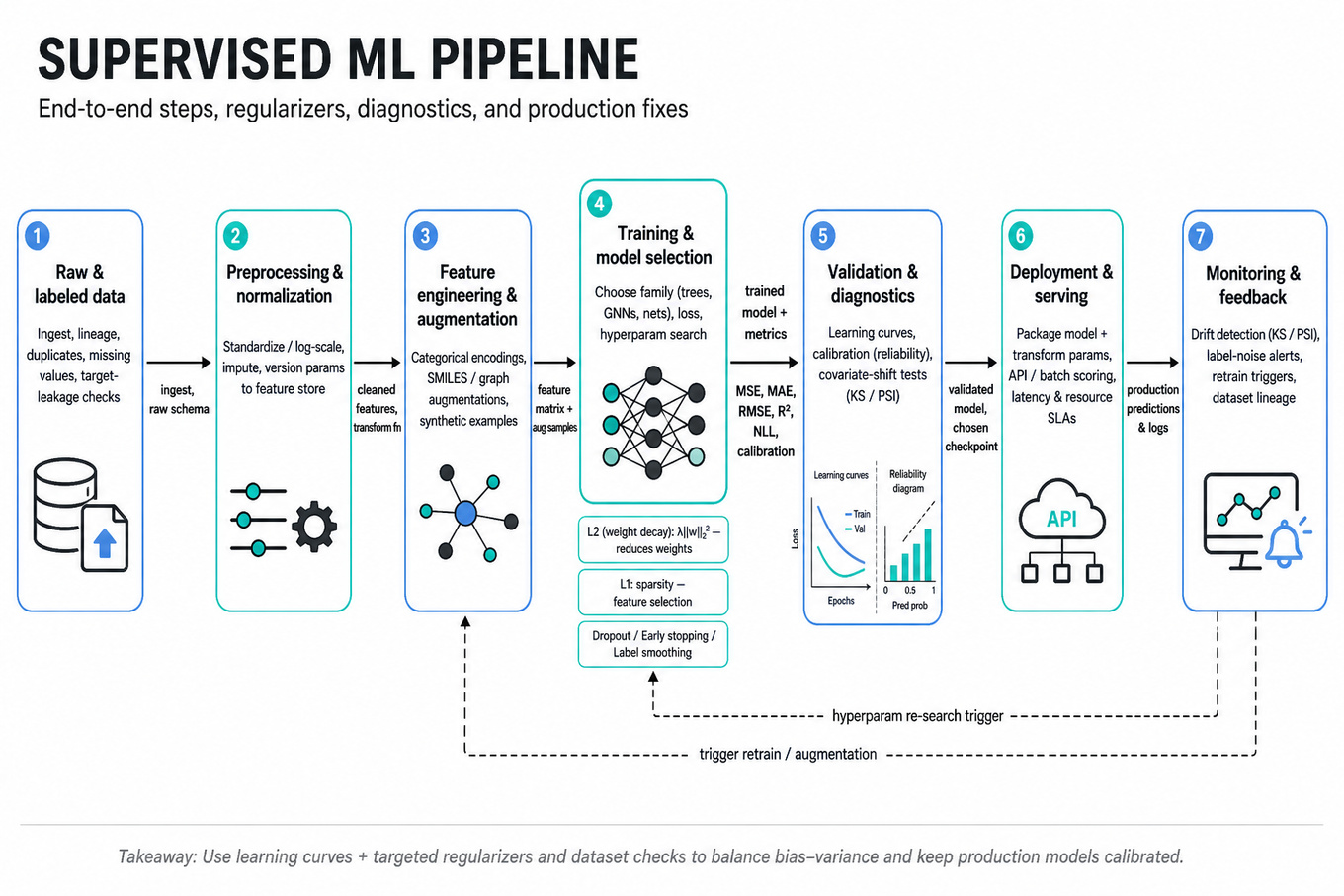
Candidates must demonstrate end-to-end supervised learning ownership: framing a regression/classification problem, choosing representations and model families, applying and reasoning about regularization, and diagnosing train/serve failures with evidence-driven fixes. Interviewers probe whether you can trade off model complexity, data-quality efforts, and monitoring needs in realistic production constraints for a Machine Learning Engineer role.

Core knowledge

• Bias–variance tradeoff: high-capacity models reduce bias but increase variance; quantify with training vs validation error curves and expected generalization gap. Use learning curves to detect which regime you’re in.

• Regularization families: L2 (weight decay) adds penalty $\lambda\|w\|_2^2$, L1 encourages sparsity, dropout stochastically removes units, early stopping is an implicit regularizer; each has different effects on interpretability and sparsity.

• Data augmentation & label smoothing: synthetic examples (e.g., SMILES augmentation, graph augmentations for molecules) increase effective data; label smoothing reduces overconfident predictions and improves calibration for classification.

• Normalization & preprocessing: apply consistent pipelines (e.g., per-feature standardization, log-scaling) offline and in serving; record and version normalization params in feature store or model artifact.

• Loss choice & metrics: regression: MSE, MAE, RMSE, and R^2; pick loss matching business utility and noise (MAE less sensitive to outliers). For probabilistic outputs, evaluate NLL, sharpness, and calibration (reliability diagrams).

• Model families & toolchain: tree models (XGBoost, LightGBM) often excel with tabular features; neural graph models (PyTorch Geometric) suit molecular graphs; calibrate choices to dataset size (trees for <10M rows, deep nets for large, structured data).

• Diagnostics for data issues: check target leakage, duplicated examples, label noise, covariate shift (compare feature distributions via KS or population stability index), and missing-value mechanisms; instrument dataset lineage so you can reproduce problematic splits.

• Hyperparameter search & validation: use nested cross-validation for model selection if dataset small; prefer a temporally-respecting holdout for time-dependent signals; budget Bayesian or asynchronous bandit search for large pipelines.

• Uncertainty decomposition: distinguish aleatoric (noise in labels) vs epistemic (model uncertainty); use ensembles, MC Dropout, or Bayesian approaches to quantify epistemic uncertainty for active retraining.

• Ensembling & calibration tradeoffs: ensembles (bagging, stacking) reduce variance but increase latency and maintenance; apply temperature scaling or isotonic regression to fix miscalibration post hoc.

• Training/serving parity & drift monitoring: ensure same preprocessing and features in training and serving; deploy data-drift and label-drift monitors, and track training/online feature distribution, prediction distribution, and downstream metric regressions.

• Regularization vs underfitting: don’t over-regularize; monitor both train and validation error. If both are high, add capacity or improve features rather than increase regularization.

Worked example — Design a reaction-factor prediction system

First 30 seconds: clarify the target (scalar reaction yield/regression or factor range), available inputs (molecular graphs, experimental conditions, dataset size, label noise), and production constraints (latency, retraining cadence). Organize your answer into four pillars: data & labeling, representation & features, model & training pipeline, and evaluation, deployment & monitoring. Data work: validate labels, deduplicate reactions, augment via chemically-valid transformations (e.g., alternate SMILES, graph augmentations), and compute domain-specific features (fingerprints, computed descriptors) stored in the feature store. Representation: evaluate both tabular (fingerprints + reaction conditions) with XGBoost and a graph neural network for pairwise molecular interactions; choose simpler model when dataset <100k examples. Training: implement weight decay, early stopping on validation RMSE, and mixup-like augmentations for regression (interpolating inputs/targets carefully only when chemically valid). Evaluation: use holdout test with scaffold-aware splits to avoid overoptimistic generalization; report RMSE, MAE, calibration plots, and uncertainty estimates via ensembles. Deployment: expose model behind a low-latency service, ensure identical preprocessing artifacts (serialize scalers/encoders), and monitor drift on reaction chemotype distributions plus downstream experimental success rates. Tradeoff to call out: complex GNNs may increase offline performance but cost latency and operational complexity — prefer a strong tree baseline plus targeted GNN for high-value predictions. Close: state you'll implement a rollout with shadow testing and A/B evaluation, then iterate on data labeling and uncertainty-driven active learning if model confidence is insufficient.

A second angle — Explain modeling challenges and fixes

Framing here shifts from design to diagnosis. Start by instrumenting: collect per-slice training/validation metrics, feature distributions, and model outputs. Common pillars are reproduce the failure, isolate cause (data/model/hyperparams/serving), then test a hypothesis (e.g., train on cleaned subset, remove suspect feature, or disable regularizer). Practical fixes include correcting label noise via human relabeling or noise-robust losses, reducing overfitting via stronger weight decay or augmentation, and restoring parity by aligning preprocessing in training and serving. Emphasize experiments that produce measurable improvements (e.g., val RMSE drop, calibration improvement) and guard against overfitting fixes to the validation set by using a fresh holdout or cross-validation.

Common pitfalls

Pitfall: confusing validation leakage with generalization — tuning hyperparameters on a test set gives optimistic estimates.

Always define separate train / validation / test sets; when performing many experiments, keep a final untouched test split or use nested CV.

Pitfall: blaming the model when the signal is missing — complex models amplify noisy labels.

If both training and validation errors are high, prioritize improving features, collecting cleaner labels, or changing loss (e.g., MAE) instead of increasing model capacity.

Pitfall: ignoring train/serve mismatch — production inputs undergo different preprocessing.

Version and serialize preprocessing artifacts (scalers, categorical maps) with the model; include end-to-end integration tests and synthetic shadow runs to validate parity.

Connections

Expect pivots to feature-store design and versioning, online learning / incremental update strategies, and model evaluation pipelines (CI for ML, continuous validation). Interviewers may also ask about deployment tradeoffs (latency vs ensemble size) or experiment design for model rollouts (ramp schedules, guardrail metrics).

Further reading

• Deep Learning — Goodfellow et al., foundational for regularization and optimization principles.

• mixup: Beyond Empirical Risk Minimization — original paper on input interpolation augmentation with practical tradeoffs.

Practice questions

Behavioral & Leadership

You viewed experimentation content once; Google expects metric and guardrail reasoning for ML product decisions.

What's being tested

Interviewers are probing whether you can design, evaluate, and defend model-driven experiments end-to-end as a Machine Learning Engineer: choose appropriate metrics, ensure statistical validity, detect instrumentation or modeling problems, and translate results into safe deployment decisions. They care that you can own the measurement pipeline (offline → online parity), reason about short- vs long-term effects, and communicate uncertainty and mitigation plans clearly to stakeholders.

Core knowledge

• Randomization/unit of assignment: pick the correct randomization unit (user, session, device, cookie) to avoid interference and preserve independence; justify choice by product causal path and frequency of interaction.

• Primary vs guardrail metrics: define one clear primary metric (e.g., CTR, CVR, revenue per DAU) and several guardrails (engagement, latency, error-rate, fairness) that must not regress; instrument both before rollout.

• Hypothesis, effect size, and power: perform sample-size calculation using the two-sample proportions formula
  $n = \frac{(Z_{1-\alpha/2}+Z_{1-\beta})^2\,(p_1(1-p_1)+p_2(1-p_2))}{(p_2-p_1)^2}$
  and state minimal detectable effect (MDE) in product-relevant terms.

• Type I/II and multiple comparisons: control Type I error (α) with pre-registration and adjust for multiple arms via Bonferroni or control False Discovery Rate (Benjamini–Hochberg) when running many metrics or segments.

• Sequential testing: if checking results repeatedly, use alpha-spending or group-sequential methods (e.g., O’Brien–Fleming) or platform-supported sequential tests; avoid naive peeking.

• Pre-launch sanity checks: run A/A tests, check sample ratio mismatch (SRM) with chi-square, verify covariate balance, and validate logging keys and feature parity between offline training and online inference.

• Offline ↔ online parity: ensure features used in training are available and identically computed at serving (feature-store parity); measure offline metrics (AUC, NDCG, calibration) and map them to online KPI expectations.

• Heterogeneous treatment effects (HTE): analyze slices and consider uplift modeling when effects vary across cohorts; correct for data-snooping by pre-specifying key subgroups or using cross-validation for discovery.

• Drift & monitoring: set alerts for input data drift (feature distribution shifts), label delay, prediction distribution shifts, and monitor model calibration, p99 latency, and error-rate in production.

• Interference and network effects: anticipate spillover (violated SUTVA) in social or shared-resource settings; use cluster or hierarchical randomization or design cluster-level experiments.

• Long-term treatment effects: plan for metrics over time (retention, lifetime value), use holdout groups or staggered rollouts, and estimate cumulative impact instead of only short-term lifts.

• Diagnosis workflow for failures: triage by (1) instrumentation bug, (2) SRM or randomization bug, (3) data-labeling issues, (4) model/feature drift, (5) real negative treatment — use canary and shadow traffic to isolate.

Tip: Pre-register the experiment (metrics, MDE, duration) and store a reproducible analysis pipeline (Jupyter/Rmarkdown) for auditability.

Worked example — "Respond to long-term concerns after A/B success"

Frame: first clarify the observed result (which metrics improved, over what duration, sample size, and which guardrails were tracked). Ask if the effect is concentrated in new users or existing users, and whether any downstream metrics (retention, complaints, latency) showed trends.

Skeleton answer pillars:

1. Validate short-run claim: check SRM, A/A tests, and instrumentation logs; re-run statistical test with pre-registered analysis and sequential-adjustment if peeking occurred.

2. Assess external validity: analyze cohorts (new vs returning users), geographical splits, and seasonality to test robustness.

3. Estimate long-term impact: run a staged rollout with holdout or randomized control for longer windows, or project retention/LTV using survival analysis.

4. Operationalize guardrails: deploy canary with rollback criteria, set monitoring dashboards for retention, support tickets, and fairness metrics.

Tradeoff to flag: a quick full rollout maximizes short-term gain but risks long-term churn; a conservative phased rollout trades speed for safety. Close: "If I had more time, I'd set randomized long-holdout groups and run uplift models to identify cohorts where the change backfires."

A second angle — "Explain modeling challenges and fixes"

Same evaluation mindset applies when debugging a deployed model: start by validating instrumentation (SRM, logging, feature parity). Organize response around (1) reproduce offline with recent data, (2) run shadow traffic to compare production inputs/predictions to offline expectations, (3) detect drift and recalibrate (e.g., Platt scaling for probabilities), and (4) implement quick mitigations (threshold adjustments, fallback models) vs longer-term fixes (retraining, feature fixes). Emphasize tradeoffs between immediate rollback (costly but safe) and targeted mitigations (safer for partial regressions). Communicate uncertainty and an evidence-backed timeline for retraining or phased redeploy.

Common pitfalls

Pitfall: Analytic tunnel vision — only reporting a single statistically significant metric.
Surface other metrics and guardrails; pre-define primary metric and publish the full set of monitored KPIs so stakeholders don’t cherry-pick.

Pitfall: Mistaking statistical significance for practical importance.
Always translate lifts into business or user-impact terms (absolute change, N-percent of users affected, projected revenue) and report confidence intervals and MDE.

Pitfall: Overlooking instrumentation and offline/online mismatch.
Don’t assume training features equal serving features; missing features or latency can cause models to fail silently — use shadow traffic and end-to-end canaries.

Connections

Interviewers may pivot to causal inference (instrumental variables, difference-in-differences), MLOps topics (canary, CI/CD for models, feature stores), or deeper fairness and bias evaluation (metric parity by subgroup), so be prepared to bridge experimentation reasoning to these adjacent areas.

Further reading

• [Online Controlled Experiments at Large Scale — Kohavi et al.] (https://exp-platform.com/kolahavi) — practical foundations and pitfalls in online experiments.

• [Design and Analysis of Experiments — Chapter on sequential testing and sample size] — concise reference for power and alpha-spending techniques.

Practice questions

No behavioral exclusion was given; prepare ownership, conflict, and impact stories in Google-style structured answers.

What's being tested

These questions probe leadership & ownership for a Machine Learning Engineer: how you take end-to-end responsibility for ML solutions while communicating tradeoffs and outcomes. Interviewers expect structured storytelling (often STAR), clear quantification of impact, technical depth about model lifecycle decisions, and evidence of cross-functional influence and learning. They also test stakeholder management when short-term wins conflict with long-term product health.

Core knowledge

• STAR: Situation, Task, Action, Result — state context quickly, your specific responsibility, concrete technical actions, and quantified outcomes (absolute and relative). Always close with learning or next steps.

• Impact quantification: Report both relative lift and absolute change (e.g., lift = (treatment - control)/control; Δ = treatment - control), and convert to business units (e.g., monthly active users, ARR).

• Experiment validity: Know A/B testing basics: confidence intervals, p-values, and pre-experiment power calculation. For two-sample continuous means: $n\approx\frac{(z_{1-\alpha/2}+z_{1-\beta})^2(\sigma_1^2+\sigma_2^2)}{\Delta^2}.$

• Short vs long-term metrics: Distinguish leading metrics (click-through rate, immediate conversions) from lagging metrics (retention, lifetime value). Propose guardrail metrics to detect regressions.

• Drift & monitoring: Describe production monitoring for data drift, model performance drift, and label-delay effects; include alert thresholds, daily dashboards, and automatic rollback triggers.

• Technical ownership scope: As an MLE, focus on training pipelines, feature reliability, offline/online parity, model serving latency, and deployment safety. Don’t design upstream ingestion infrastructure.

• Tradeoff framing: Explicitly weigh tradeoffs: model complexity vs latency, offline evaluation fidelity vs cost of online experiments, and short-term metric lift vs long-term retention.

• Cross-functional collaboration: Name stakeholders: PMs for success criteria, SRE/infra for serving constraints, data scientists for experiment design, and legal/ethics for fairness/privacy considerations.

• Failure & blameless postmortem: Show structured root-cause (hypothesis → evidence → fix), corrective actions, and what instrumentation would prevent recurrence.

• Prioritization under change: Use clear criteria: user-impact × probability × cost/time-to-fix. Explain how to re-scope MVP vs polish work and communicate tradeoffs to stakeholders.

Worked example — Describe your proudest project

First 30 seconds: ask clarifying questions: "What metric mattered most? Who were the stakeholders? What constraints (latency, privacy, SLAs) existed?" Frame your answer around ownership (you vs team), scale, and measurable impact. Organize the story into four pillars: problem & constraints, technical approach, deployment/monitoring, and impact + lessons. Describe the model choice and why — e.g., chose LightGBM for structured features because of interpretability and low inference latency versus a deep model that would violate a 50ms p99 latency SLA. Explicitly state a tradeoff: prioritized maintainability and offline/online parity over marginal accuracy gains. End with quantified results (absolute metric change and business conversion), and close with “if I had more time, I’d A/B test a representation-learner and expand monitoring to cohort-level drift detection.”

A second angle — Respond to long-term concerns after A/B success

Start by reframing: distinguish the immediate experiment signal from potential delayed harms. Propose two concrete actions: (1) implement extended cohort analysis to measure retention and engagement over 30–90 days, and (2) add guardrail metrics (e.g., DAU, average session length, complaint rate) and segments (new users vs power users). Discuss statistical power for detecting delayed effects and the need for pre-registration of analysis to avoid p-hacking. Flag operational steps: schedule rolling evaluations, add automated alerts for negative trend detection, and consider a phased rollout or monitor-only canary to reduce risk while collecting long-term data.

Common pitfalls

Pitfall: Reporting only relative percentages without baseline or absolute numbers.
If you say “we increased CTR by 20%,” also state baseline (e.g., from 2% to 2.4%) and the practical downstream effect (additional conversions per week).

Pitfall: Deflecting responsibility or blaming others.
Interviewers expect ownership. Say “I owned X, coordinated Y” and describe how you influenced others; avoid “the team did” without clarifying your role.

Pitfall: Surface-level metrics without technical depth.
Don’t stop at “we trained a model.” Explain the actual decisions — feature validation, offline-to-online parity checks, A/B guardrails, and monitoring that ensured the result persisted.

Connections

Interviewers may pivot to experimentation design (sequential testing, multiple comparisons), model serving & ML infra (rollout strategies, canaries, model versioning), or product analytics (cohort analysis, causal inference). Be ready to show the same ownership across those adjacent domains.

Further reading

• Ron Kohavi et al., “Online Controlled Experiments at Large Scale” — practical guidance on experiment design, guardrails, and pitfalls.

• Chip Huyen, Designing Machine Learning Systems — concrete patterns for production ML pipelines and monitoring.

• STAR interview technique — Harvard Business Review summary — concise guidance on structuring behavioral answers (search “STAR method HBR”).

Practice questions

Statistics & Math

Probability appears in both ML and coding screens; no strength signal is available, so keep standard coverage.

What's being tested

These problems test discrete probability reasoning (hitting/absorbing probabilities in 1D random walks) and practical weighted sampling implementations for both batch and streaming settings. Interviewers probe whether you can convert probabilistic recurrences to computable algorithms and choose numerically stable, performance-appropriate samplers for production ML pipelines.

Patterns & templates

• Gambler's ruin / linear recurrence — write recurrence for hitting probability, solve closed-form when step distribution simple; reduce to tridiagonal linear system for general neighbors.

• Martingale / optional stopping — use expected value invariants to derive absorption probabilities when applicable.

• Prefix-sum CDF + binary search — build prefix sums O(n) and sample with O(log n) per draw via bisect; watch inclusive/exclusive indices.

• Alias method — Alias method gives O(1) draws after O(n) preprocessing; memory O(n) and numerically sensitive to tiny weights.

• Weighted reservoir (A-Chao) — streaming weighted sampling maintenance in one pass, O(1) per item amortized, handles unbounded streams.

• Numerical stability — normalize using sums in double or operate in log-space for extreme weights; avoid subtractive cancellation.

• Determinism — seed local RNGs (random.Random(seed)) for reproducible generators; avoid global random.seed() in multi-threaded services.

Common pitfalls

Pitfall: assuming finite state or symmetric steps without asking — leads to wrong closed-form for asymmetric dice or unbounded walks.

Pitfall: building CDF with floats and then using random.random() without normalization — can sample out-of-range for tiny/huge totals.

Pitfall: returning first non-zero weight when all weights zero or negative — always validate and define behavior for zero/negative weights.

Practice these

the practice cards below cover the canonical variants — solve all of them and time yourself.

Practice questions