Meta Data Scientist Interview Prep Guide

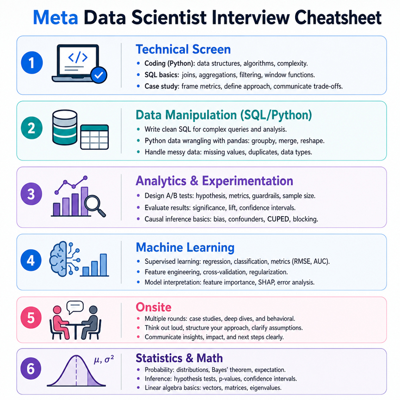
Focus most on experiment design under interference, power/MDE, diagnostics, metric design, causal inference, delayed outcomes/censoring, and ML ranking/fraud topics; many of your chosen concept ratings are shaky or new there. Merely review core SQL event-log mechanics and Bayesian/base-rate probability at a normal pace, since you viewed SQL/statistics content but did not explicitly mark those as gaps. The Meta-specific emphasis is ads measurement, Facebook/Instagram surface metrics, Messenger networked adoption, commerce visibility, recommendations, and trust/safety fraud. With one month left and mid-level self-ratings across analytics, stats, and ML, plan roughly 90 minutes per technical-screen pass and 100 minutes per onsite pass.

Technical Screen — 87 min

Data Manipulation (SQL/Python)

• Shop Visibility And Commerce Analytics (Focus) — covered in depth under Onsite below.

Analytics & Experimentation

• A/B Testing And Experiment Design (Focus) — covered in depth under Onsite below.

• Network Effects And Cluster Randomization (Focus) — covered in depth under Onsite below.

• Product Metrics, Trade-Offs, And Communication (Focus) — covered in depth under Onsite below.

• Messenger, Group Calling, And Networked Adoption (Focus) — covered in depth under Onsite below.

• Facebook And Instagram Product Surface Analytics (Focus) — covered in depth under Onsite below.

• Observational Causal Inference For Meta Products (Focus) — covered in depth under Onsite below.

• Delayed Outcomes, Censoring, And Survival Analysis (Focus) — covered in depth under Onsite below.

Machine Learning

• Trust, Safety, Fake Accounts, And Fraud (Focus) — covered in depth under Onsite below.

• Time-Series Forecasting For Product Metrics (Focus) — covered in depth under Onsite below.

• Tree Ensembles And XGBoost For Tabular ML (Focus) — covered in depth under Onsite below.

• Missing Data, Imputation, And Selection Bias (Focus) — covered in depth under Onsite below.

Onsite — 96 min

Data Manipulation (SQL/Python)

Focus area — Commerce and marketplace metrics connect to your selected funnel, attribution, and two-sided experiment topics, plus Meta shopping surfaces.

What's being tested

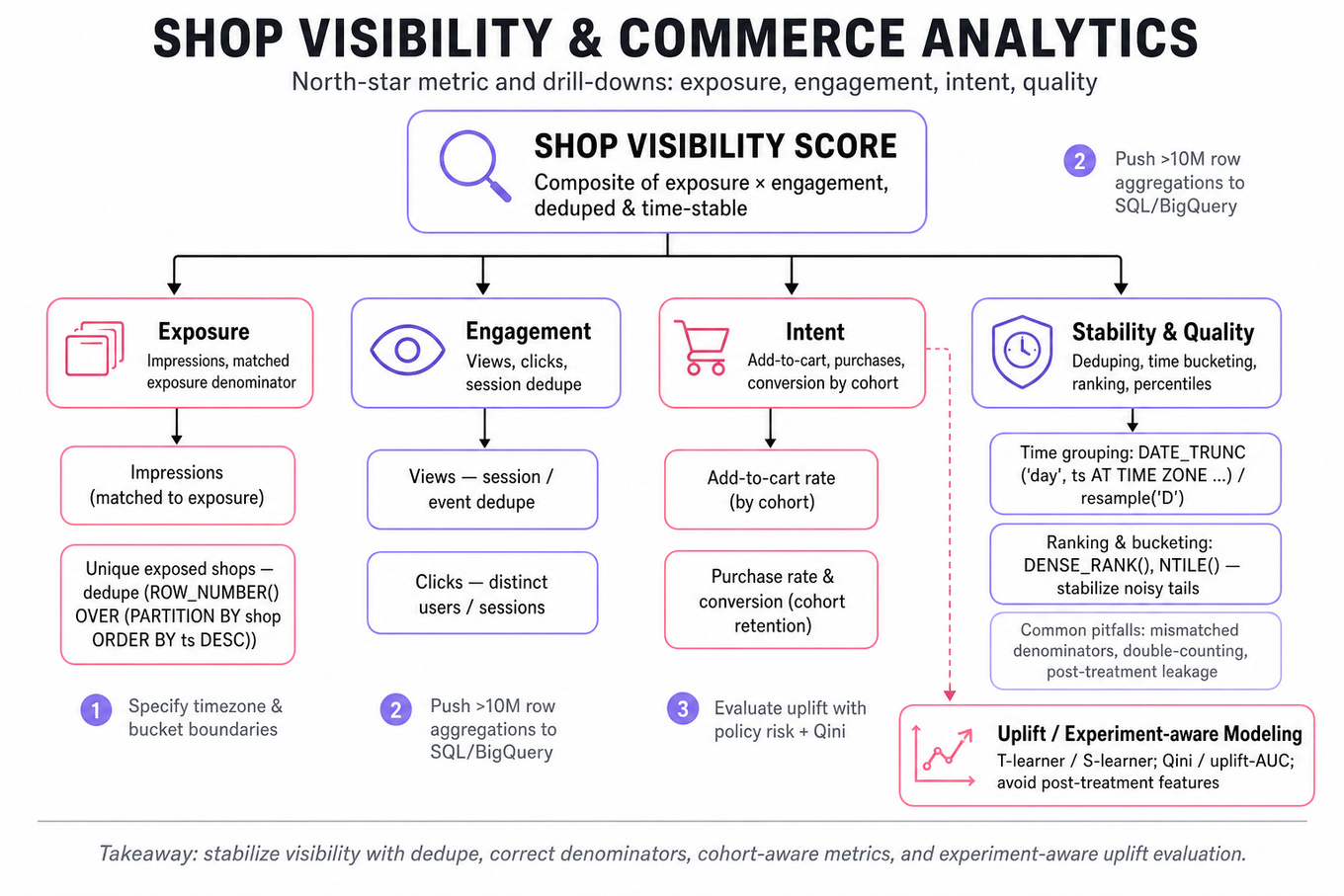
Tests the ability to run cohort analysis and time-series aggregation to quantify shop visibility, apply dedup/ranking logic, and design stable visibility/intent metrics. Also probes experiment-aware modeling and uplift modeling for causal buyer-engagement decisions.

Patterns & templates

• Window functions for deduping and last-event logic — `ROW_NUMBER()` OVER (PARTITION BY shop ORDER BY ts DESC); tie-break with deterministic id.

• Time-based grouping using `DATE_TRUNC('day', ts AT TIME ZONE ...)` or `ts::date`; always specify timezone and bucket boundaries.

• Conditional aggregation idiom: `SUM(CASE WHEN event='view' THEN 1 ELSE 0 END)` or `COUNT(DISTINCT CASE WHEN ... END)`; use `FILTER` when available.

• Cohort assignment: compute `first_seen_date` per shop, then join a calendar of relative days to measure retention/decay across cohorts.

• Ranking & percentiles: `DENSE_RANK()` or `NTILE()` over visibility metric; report distribution buckets to stabilize noisy tails.

• Uplift modeling templates: T-learner / S-learner or meta-learners; evaluate with Qini/ uplift-AUC and policy risk, avoid post-treatment features.

• pandas performant idioms: `df.groupby(['shop','date']).agg(...)`, `resample('D')`; push heavy aggregations back to `SQL`/`BigQuery` for >10M rows.

Common pitfalls

Pitfall: Using impressions as denominator then comparing to views without matching exposure leads to biased visibility ratios.

Pitfall: Double-counting events across overlapping time-windows or failing to dedupe session-level events inflates metrics.

Pitfall: Training an uplift model using post-treatment features or leaking future exposure produces overly optimistic policy estimates.

Practice these

The practice cards below cover the canonical variants — solve all of them and time yourself.

Practice questions

Analytics & Experimentation

Focus area — You selected A/B testing, power/MDE, diagnostics, and several related concepts are shaky or new, so this needs priority practice.

What's being tested

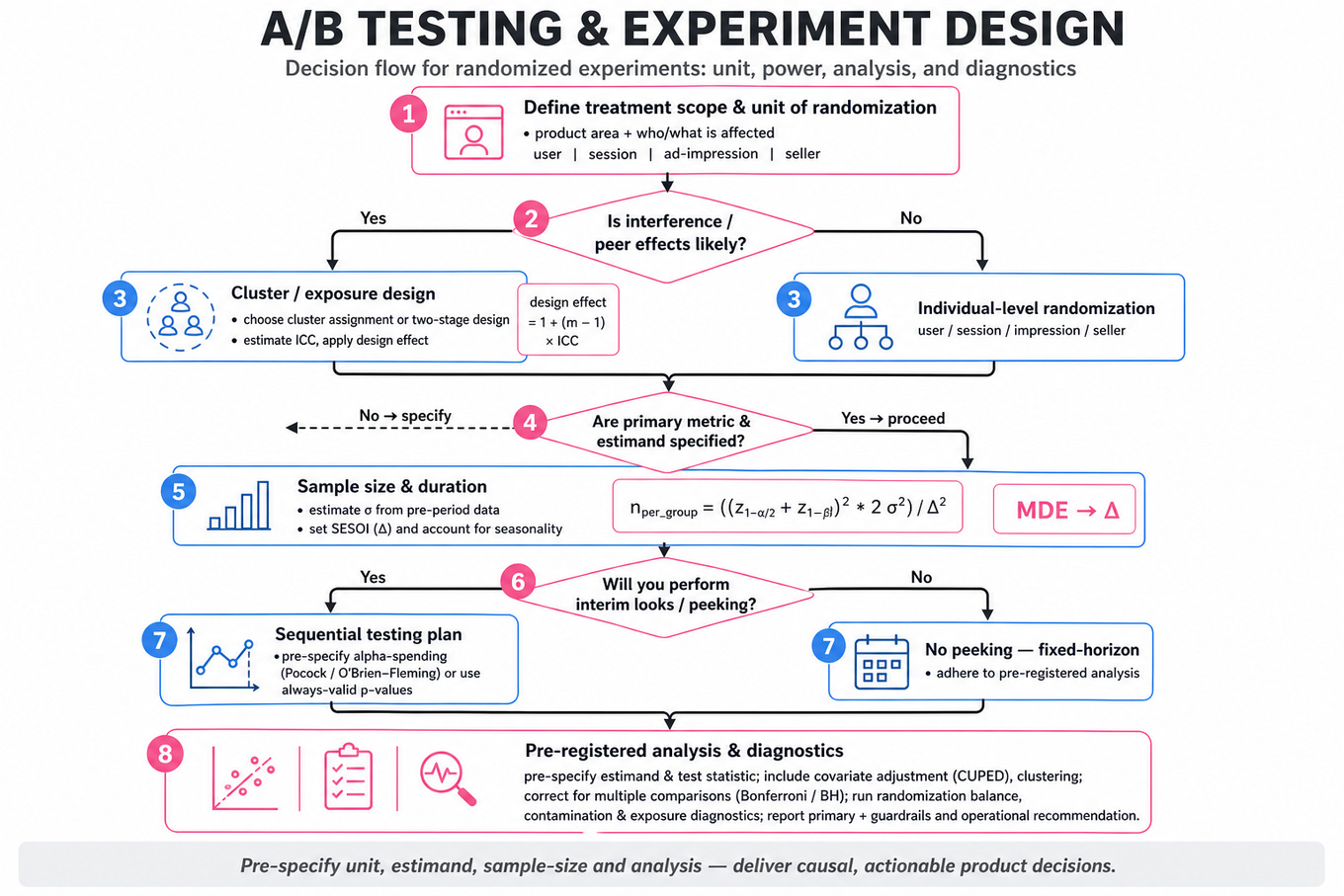
Candidates must demonstrate end-to-end mastery of randomized experiment design and analysis for product decisions: choosing the correct unit of randomization, defining primary and guardrail metrics, computing sample sizes and power, and producing a pre-registered analysis that handles clustering, covariate adjustment, and possible interference. Interviewers probe statistical reasoning (Type I/II tradeoffs, sequential testing), practical variance-reduction techniques (e.g., CUPED), and operational diagnostics for ambiguous or null results. The goal is to show you can deliver a causal, defensible answer a product team can act on.

Core knowledge

• Randomization unit: choose between user, session, ad-impression, or seller based on treatment scope and interference; wrong unit creates contamination or underpowered experiments.

• Hypotheses & estimand: state null/alternative and exact estimand (e.g., average treatment effect on users who see the new algorithm), not just “does it improve CTR”.

• Sample-size formula: for two-sample mean test, per-group n = ((z_{1-α/2}+z_{1-β})^2 * 2σ^2) / Δ^2; estimate σ from pre-experiment data and set minimum detectable effect Δ (SESOI).

• Power tradeoffs: doubling sample reduces detectable Δ by √2; longer duration vs. larger population—account for seasonal/weekday patterns when estimating duration.

• Cluster randomization & ICC: design effect = 1 + (m−1)*ICC inflates required sample when randomizing clusters; estimate intraclass correlation (ICC) from historical data.

• Covariate adjustment / CUPED: subtract linear projection on baseline covariate to reduce variance; works best when pre-period metric correlates strongly with outcome (use regression-based adjustment in R/Python).

• Sequential testing & peeking: avoid naive peeking; use alpha-spending (Pocock/O’Brien–Fleming) or validated sequential methods (e.g., always-valid p-values) to preserve Type I error.

• Multiple comparisons: correct for familywise error when testing many variants/metrics (Bonferroni, Holm) or control FDR (Benjamini–Hochberg) and predefine metric hierarchy (primary vs. guardrails).

• Interference & exposure models: if SUTVA violated, define exposure mapping (who is exposed to treated peers) and consider cluster assignment, two-stage randomization, or partial population designs.

• Analysis plan: pre-specify estimand, test statistic, transformation (log, winsorize), outlier handling, and whether to use cluster-robust SE, permutation tests, or bootstrapping for inference.

• Guardrails and safety metrics: always include business guardrails (e.g., revenue, retention, quality signals) and health metrics (latency, error rate); use sequential monitoring but mute decisions until final.

• Null results interpretation: distinguish low power from true null with confidence intervals, equivalence testing, and reporting of minimal detectable effects; quantify uncertainty for product decisions.

• Diagnostics: randomization checks, instrumentation loss, skewed traffic splits, and differential attrition; check balance on pre-period metrics and stratify or reweight if needed.

Worked example — "Design an A/B test for a new shop-ads algorithm"

First 30 seconds: ask clarifying questions — what’s the treatment (ranking model change?), scope (all shoppers or subset?), cost of misassignment, and primary business metric (e.g., ad revenue per DAU vs. purchase conversion). State assumptions: stable traffic, instrumentation available via BigQuery logs, pre-period metric for CUPED. Organize the answer into pillars: (1) unit of randomization — randomize at user to avoid the same shopper seeing mixed algorithms (unless seller-level constraints force clustering), (2) metrics — primary: revenue per user (log-transform), guardrails: CTR, purchase-rate, organic engagement, (3) power/sample-size — compute n using historical σ and SESOI, inflate for expected ICC or baseline variability, (4) analysis plan — pre-register intent-to-treat ATE, use CUPED with pre-period revenue, apply cluster-robust SE if clusters used, (5) monitoring & roll-out — limited ramp, abort thresholds tied to guardrails. Flag a tradeoff: randomizing at seller vs. user trades statistical efficiency for reduced interference; state rule-of-thumb: prefer user-level unless seller-level interference is large. Close with next steps: if time allowed, plan heterogeneous treatment effect analysis by cohort, long-term retention measurement, and an uplift model to personalize decisions.

A second angle — "Design and analyze an A/B test with interference"

Interference forces you to redefine the estimand: instead of ATE assume partial interference and specify spillover estimands (direct vs. indirect effects). Use cluster randomization (e.g., households, social-graph clusters) or two-stage randomization to estimate spillovers explicitly. If clusters are impractical, build an exposure model mapping which users are plausibly affected and analyze conditional ATEs (those exposed vs. not). Analysis-wise, rely on permutation tests respecting cluster boundaries or use randomization inference to get valid p-values under interference. The same fundamentals (power, pre-specification, guardrails) apply, but sample-size must account for between-cluster variance and the loss of effective sample due to contamination.

Common pitfalls

Pitfall: Ignoring clustering. A tempting quick-sample calculation assuming i.i.d. users will understate required sample when ICC>0; always estimate ICC and apply the design effect to sample-size.

Pitfall: Over-interpreting p-values from a peeked experiment. Early peeking without sequential corrections yields inflated Type I error; report always-valid intervals or use pre-defined stopping rules.

Pitfall: Reporting a null as “no effect” without SESOI. A non-significant result might be underpowered; present the confidence interval and whether it excludes the smallest effect size of interest.

Connections

Interviewers may pivot to heterogeneous treatment effect estimation (uplift models) or to observational causal inference methods when randomization isn’t feasible. They may also ask about experiment-velocity infrastructure (monitoring plans, but not pipeline internals), or ML model evaluation for ranking metrics.

Further reading

• Kohavi et al., "Online Controlled Experiments at Large Scale" — practical lessons from industry on design and pitfalls.

• Deng, Lu, and Kohavi, "Improving Online Controlled Experiments with Variance Reduction" (CUPED) — technique and empirical guidance.

• Hudgens & Halloran, "Toward Causal Inference With Interference" — formal treatment of interference and estimands.

Practice questions

Focus area — Interference, cluster randomization, SUTVA, exposure mapping, and graph clustering are marked shaky or new.

What's being tested

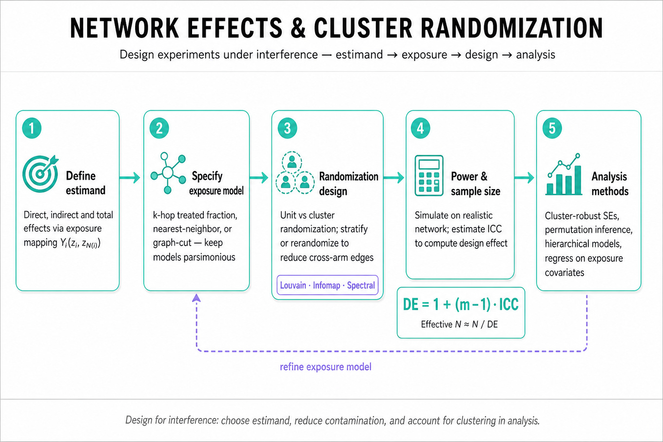
These prompts evaluate a candidate's ability to design and analyze experiments when interference (units affecting each other) breaks the usual A/B test assumptions. Interviewers probe whether you can define a clear estimand, construct an exposure model, pick a randomization strategy (unit vs. cluster randomization), and quantify power and bias under spillovers. Meta cares because social products have strong network effects; a Data Scientist must measure causal impact while controlling contamination, false precision, and rollout risk.

Core knowledge

• Interference / spillover: occurs when one unit’s treatment affects another’s outcome; this violates SUTVA and requires explicit exposure mapping (e.g., treated fraction in neighborhood) to define causal effects unambiguously.

• Estimand types: average treatment effect (ATE) is insufficient; define direct, indirect (spillover), and total effects. Use potential-outcomes with exposure mapping: $Y_i(z_i, z_{N(i)})$.

• Exposure models: operationalize interference using k-hop treated proportion, nearest-neighbor treated indicator, or graph-cut exposures; choose parsimonious models to avoid combinatorial explosion of potential exposures.

• Cluster randomization: randomize connected subgraphs to treatment or control to reduce cross-arm edges; cluster size (m) and number (K) trade power vs. contamination risk; prefer many small clusters when ICC is low.

• Design effect and ICC: adjust variance by design effect $DE = 1 + (m-1)\,ICC$. Effective sample size ≈ $N/DE$. Estimate ICC from historical metrics or pilot.

• Graph clustering algorithms: use Louvain, Infomap, or spectral clustering to produce clusters; balance edge-cut minimization with cluster size constraints to avoid very large clusters that reduce power.

• Randomization schemes: cluster-level (reduces contamination), stratified (by community size or pre-period metric), and graph-based rerandomization (reject assignments with many cross-arm edges) are common; log computational cost for large graphs.

• Analysis methods: use cluster-robust SEs, permutation / randomization inference on clusters, and hierarchical models to separate within-cluster and between-cluster variability; for exposure models, estimate via regression with exposure covariates and robust SEs.

• Power & sample size: simulate using realistic network and behavior models; analytic approximations use $Var(\bar{Y}) \approx \sigma^2/(n\cdot p(1-p))\cdot DE$ for difference-in-means, adjusting for binary/zero-inflated outcomes and expected effect heterogeneity.

• Contamination and routing: measure cross-arm interactions post-hoc with edge-level logs (message edges, payment flows); quantify contamination rate and bias direction to inform rollout decisions and guardrails.

• Inference under interference: consider partial interference assumptions (clusters independent) or use randomization-based inference (permutation within cluster-assignments) when asymptotics are fragile.

• Safety & guardrail metrics: for monetization features (ARPU, fraud rate) include short windows for safety, pre-specified stopping rules, and correction for multiple looks (e.g., alpha-spending) when sequential monitoring is needed.

Worked example — "Design cluster-randomized test under network effects"

First 30 seconds: clarify the estimand (direct effect on treated users? total effect including spillovers?), define allowable exposure (e.g., treated user with ≥1 treated friend), and constraints (graph size, rollout risk). Skeleton answer pillars: (1) construct clusters by minimizing cross-arm edges using Louvain with size caps; (2) randomize clusters stratified by pre-period metric and cluster size; (3) specify estimands and exposure mappings and plan analysis (cluster-level difference-in-means + randomization inference); (4) run power sims under varying ICC and contamination; (5) define guardrails and monitoring. Key tradeoff: larger clusters reduce contamination but increase DE and reduce power — explicitly quantify via $DE=1+(m-1)ICC$ and show how many clusters needed for target power. Close by saying: if more time, I'd run synthetic-network simulations calibrated to historical interaction rates, test alternative exposure mappings, and prepare post-hoc diagnostics for contamination and heterogeneous effects.

A second angle — "Design and evaluate P2P payments in messaging"

The same interference concerns appear but monetization and fraud elevate priorities. Here the estimand often includes ARPU change and risk metrics (fraud rate, chargebacks). Network pathways (who pays whom) are directional, so exposure models must account for sender vs receiver roles. Cluster construction should preserve natural payment subgraphs (frequent payer-recipient pairs) and avoid splitting payment dyads across arms. Power sims must incorporate heavy-tailed payment amounts and low event rates; consider zero-inflated outcome models. Analysis should add outcome transformations (log or winsorization) and pre-specified subgroups (high-value transactors). Operationally, include conservative safety stops and offline fraud scoring as guardrails.

Common pitfalls

Pitfall: Over-simplifying interference to "ignore it" and running a unit-randomized A/B test — this yields biased estimates when cross-arm edges are non-negligible; always quantify expected contamination.

Pitfall: Treating cluster construction as a black box — using Louvain without size constraints can create a few giant clusters that kill power via high DE; present alternative clusterings and show sensitivity.

Pitfall: Reporting naïve p-values without accounting for cluster-level randomization or exposure mapping — use cluster-robust SEs or randomization inference and explicitly state the inferential assumptions.

Connections

Interviewers may pivot to causal graph identification, heterogeneous treatment effects (HTE) across network positions, or to implementation metrics like logging edge-level exposures in Postgres or event streams. They might also ask about simulation pipelines to calibrate power for graph experiments.

Further reading

• Ugander et al., "Graph Cluster Randomization" — practical cluster construction ideas for experiments on networks.

• Hudgens & Halloran, "Interference and Causal Inference" — foundational theory for partial interference and estimands.

Practice questions

Focus area — Metric design concepts like denominators, guardrails, decomposition, ratio metrics, and unit of analysis are marked shaky.

What's being tested

These prompts probe a Data Scientist's ability to design, analyze, and communicate product experiments and metrics where causal inference, metric design, and product trade-offs interact. Interviewers want to see that you can pick the right unit of analysis, quantify both direct lift and indirect effects (spillovers/cannibalization), set up defensible hypothesis tests and power calculations, and translate uncertainty into a clear recommendation for launch decisions. At Meta scale, this also means balancing statistical rigor with business constraints and cross-functional clarity.

Core knowledge

• Unit of randomization: Randomize at the level that prevents interference; individual-level when SUTVA holds, cluster randomization (e.g., by group, thread, or region) when interference or cross-account cannibalization exists; cluster tests reduce effective sample size and require ICC-aware power calcs.

• Spillover / interference: Understand SUTVA violations and estimate spillovers using exposure models (e.g., partial interference assumptions) or explicit network-cluster experiments; report direct, indirect, and total effects.

• Metric hierarchy: Define one primary (north‑star) metric, 2–5 secondary metrics, and multiple guardrails (safety/quality). Primary must be interpretable, powerable, and aligned to business objective.

• Ratio metrics & denominators: For rate metrics (e.g., reactions per message) track denominator stability; use delta-method or bootstrap for CI when denominators vary. Avoid misleading per-session normalization when sessions differ across groups.

• Power & MDE: Use power formula for difference in means: $n = 2\sigma^2 (z_{1-\alpha/2}+z_{1-\beta})^2/\Delta^2$; for clustered tests scale variance by design effect $DE = 1 + (m-1)\rho$ where $\rho$ is ICC.

• Multiple testing & FDR: For many segments/metrics use Benjamini–Hochberg to control false discovery rate; reserve a single pre-registered primary metric to avoid alpha leakage; consider hierarchical testing.

• Sequential testing: If analyzing repeatedly, use alpha-spending or sequential methods (e.g., O’Brien–Fleming, Bayesian credible intervals) to avoid inflated Type I error.

• Cannibalization quantification: Compare per-account lift vs cross-account displacement by measuring absolute counts and relative shares; design experiments to observe both treated and untreated recipients to estimate net system-level impact.

• Heterogeneous effects & segments: Pre-specify segmentation (new vs. power users, region, group-size) and test interaction terms; beware post-hoc slicing without FDR correction.

• Short-term vs long-term effects: Report immediate engagement lift and retention/decay curves; compute cumulative lift over meaningful horizon and discount future effects if required.

• Causal estimands: Distinguish ITT (intention-to-treat) from ATT (treatment-on-treated) and when to use each; for partial exposure, instrument with assignment to get unbiased causal effects.

• Communication & decision criteria: Present point estimates, CIs, and upside/downside scenarios (best/worst plausible impacts), and recommend threshold-based actions (launch, iterate, kill) tied to product and safety guardrails.

Worked example — Communicate trade-offs and influence launch

First 30 seconds: clarify the primary objective (growth, engagement, revenue), the unit of measurement (per-account, per-content), and whether treatment exposure could affect other accounts (possible cannibalization). Skeleton: (1) define metric hierarchy (primary uplift, secondary engagement, guardrails like abuse rate); (2) quantify per-account uplift with CIs and statistical power; (3) estimate cross-account cannibalization via exposure patterns or cluster arms and compute net system impact; (4) present uncertainty and business trade-offs (e.g., small per-account lift but large aggregate loss). Key tradeoff to flag: cluster randomization reduces interference but inflates sample requirements — you must balance measurement fidelity with time-to-decision. Close by proposing next steps: if results borderline, run an expanded cluster or network experiment, instrument downstream signals, and simulate long-term retention impacts.

A second angle — Evaluate emoji reactions launch

Same principles apply but constraints differ: social/messaging features create high potential for network effects and compositional changes (reactions may shift activity from commenting to reacting). Frame the answer around causal attribution: pick primary metric (net messages+reactions per DAU), guardrails (toxicity, moderation load), and a design that captures both sender and recipient effects (two-way randomized exposure or randomize on threads). Pay attention to denominator shifts: if users reply less but react more, absolute engagement may be constant. Use mediation-style analysis to decompose direct product usage lift vs reallocation across channels, and recommend launch only if net system engagement or retention effect is positive and safety guardrails hold.

Common pitfalls

Pitfall: Ignoring interference by randomizing at the wrong unit — leads to biased uplift estimates and overconfident conclusions. Always ask how treatment can affect non-treated users.

Pitfall: Reporting only relative lifts without absolute counts — a 10% lift on a tiny baseline can be immaterial; always show both percent and delta in absolute units.

Pitfall: Overstating certainty — presenting a single-point estimate to executives without CIs, power context, or downside scenarios undermines trust. Frame recommendations with clear thresholds and contingencies.

Connections

Interviewers may pivot to segmentation and cohort analysis (how effects vary by user cohort), longitudinal retention modeling (survival curves, churn hazard), or uplift modeling (personalization decisions based on heterogeneous treatment effects).

Further reading

• Kohavi, Longbotham — Online Controlled Experiments at Large Scale (KDD/Book chapters) — practical guidance on large-scale A/B testing and pitfalls.

• Aronow & Samii — Estimating Average Causal Effects Under Interference (article) — technical treatments of spillovers and partial interference.

• Evan Miller — Statistics for A/B Testing (guide) — clear, pragmatic explanations of power, MDE, and ratio metrics.

Practice questions

Focus area — Networked adoption and interference topics you flagged show up directly in Messenger/group calling experiments.

What's being tested

These prompts probe a Data Scientist's ability to design and analyze experiments and observational analyses where network effects / interference matter: picking the right unit of randomization, defining an Overall Evaluation Criterion (OEC) that captures primary and spillover value, and using statistical methods robust to correlated outcomes (clustered or networked). Interviewers want to see causal reasoning (how to estimate direct vs indirect effects), pragmatic power/sample-size calculations with ICC or design effect adjustments, and concrete analysis plans (pre-specification, guardrails, monitoring).

Core knowledge

• Interference / spillovers: interference violates SUTVA; treatment for one unit can change others' outcomes. Distinguish direct, indirect, and total effects (Hudgens & Halloran-style framing) when writing hypotheses.

• Unit of randomization choices: individual randomization (max power, high contamination risk) vs cluster randomization (reduced contamination, lower effective N). Decide using network topology and cross-cluster edge volume.

• Design effect & ICC: adjust sample size for clustering using design effect: $DE = 1 + (m-1) \cdot ICC$ where $m$ is average cluster size. Effective sample size ≈ $N/DE$.

• Graph cluster randomization: partition users with community detection (e.g., Louvain, METIS) or edge-cut minimization to keep most edges intra-cluster; balance cluster sizes to control power loss.

• Exposure models: summarize a user's neighborhood treatment as features (e.g., fraction of friends treated, count of treated neighbors, time-weighted exposure) and pre-define thresholds or continuous models for indirect-effect estimation.

• Randomization inference / permutation tests: with interference, use randomization-based p-values (shuffle cluster assignments consistent with design) to get exact-type I error control when asymptotics fail.

• Metric design (OEC and guardrails): pick a single OEC (e.g., weekly unique group-call participants per DAU) plus guardrails (call quality p99 drop, spam flags, support tickets, ARPU). Pre-specify secondary metrics and multiplicity control (Benjamini–Hochberg or hierarchical testing).

• Power for count/rare events: use Poisson or negative-binomial models and simulate power when base rates are low; analytic approximations fail for sparse outcomes or highly skewed cluster sizes.

• Observational log analysis patterns: dedupe sessions with ROW_NUMBER() OVER (PARTITION BY user ORDER BY ts DESC) for last event, sessionize with idle-time thresholds, and build pair-unique interactions using canonical (min,max) ID tuples.

• Causal identification strategies: if randomization infeasible, use instrumental variables (encouragement designs), difference-in-differences with parallel-trends checks, and regression with network-fixed effects or cluster-robust SEs.

• Monitoring and stopping rules: pre-specify interim checks for guardrails, use alpha-spending or sequential testing frameworks (e.g., O’Brien–Fleming), and avoid peeking on OEC without adjusted thresholds.

Worked example — Design and analyze a group-calls experiment

First 30s: ask what success looks like (engagement, retention, revenue), constraints (can we randomize at cluster level?), and expected network structure (average degree, existence of tight friend groups). Skeleton answer pillars: (1) randomization unit and clustering algorithm (graph-cluster randomization using Louvain to keep edges internal), (2) OEC and guardrails (weekly unique call participants per DAU; guardrails: call drops, spam rate, support tickets), (3) analysis plan accounting for interference (estimate direct vs indirect effects via exposure models; use randomization inference for p-values), (4) power and monitoring (simulate with observed degree distribution; compute DE using ICC estimate). Key tradeoff to flag: larger clusters reduce contamination but inflate design effect and reduce power — quantify by simulating effective sample size. Close with next steps: run a pilot A/A to validate logging and ICC, simulate treatment diffusion, and pre-register analysis plan with multiple-hypothesis controls.

A second angle — Analyze Recent User Activity from Video Call Logs

This is observational aggregation rather than randomized inference, but the same network concerns appear as features. First clarify retention windows (7/28/90-day), canonicalize IDs (account vs device), and define what counts as an interaction (joined > X seconds). Skeleton: (1) SQL dedupe using ROW_NUMBER() to get last activity per user; (2) compute unique pair interactions with canonical (LEAST(user1,user2), GREATEST(...)); (3) generate exposure covariates (num unique contacts in last 7 days) to use as predictors in downstream models. Differences: causal claims are limited without exogenous variation — use quasi-experimental methods (instrumental variables, regression discontinuity if available) or treat outputs as diagnostics for experiment design (estimate ICC, degree distributions, baseline rates) to power future randomized tests.

Common pitfalls

Pitfall: Treating users as independent in analysis — ignoring clustering/interference underestimates variance and will inflate false positives. Always compute cluster-robust SEs or use randomization inference.

Pitfall: Vagueness about the OEC — proposing many primary metrics or leaving guardrails unspecified leads to post-hoc selection. Pre-specify one OEC, ranked secondaries, and multiplicity rules.

Pitfall: Over-relying on analytic power formulas without simulation — skewed cluster-size distributions, low base rates, or overdispersion break closed-form approximations; simulate using the real network and event-rate assumptions.

Connections

Interviewers often pivot to adjacent topics: A/B testing for spam / safety where clustering preserves attacker behavior, or monetization experiments (ARPU uplift from in-call purchases) which layer revenue attribution on the same network-aware framework. They may also move toward recommendation/ranking impacts on call invitations and downstream engagement.

Further reading

• Hudgens, M. G. & Halloran, M. E. — "Toward causal inference with interference" — formal definitions of direct/indirect effects and randomized designs under interference.

• Ugander et al. — "Graph cluster randomization" (conference/paper) — practical methods to partition networks for cluster-level experiments and reduce bias from spillovers.

Practice questions

Focus area — This anchors Meta-specific product sense across Feed, Stories, Groups, Checkout, Dating, and cross-app trade-offs.

What's being tested

Interviewers are probing the candidate's ability to design, evaluate, and interpret product analytics and experiments for feed-surface recommendations (e.g., restaurant suggestions) using limited, privacy-sensitive signals. Expect to demonstrate experiment design, metric hierarchy and guardrails, causal inference (including unit-of-randomization and spillovers), and evaluation of ranking quality and business impact. Meta cares because these features affect user engagement, long-term retention, platform health, and partner fairness; the DS must balance statistical rigor with product constraints (privacy, sampling, battery).

Core knowledge

• Metric hierarchy: define one primary business metric (e.g., incremental bookings or reservation conversions) plus secondary engagement metrics (CTR, session length) and guardrail metrics (feed health, DAU, complaint rate). Always state directionality and acceptable deltas.

• Unit-of-randomization & SUTVA: randomize at the level that avoids interference; candidate units: user, session, geographic cluster. Explicitly address spillovers and violations of SUTVA (e.g., friends influencing each other).

• Power & sample-size: know two-sample formulas; for proportions: $n \approx \frac{(Z_{1-\alpha/2}+Z_{1-\beta})^2 [p_0(1-p_0)+p_1(1-p_1)]}{(p_1-p_0)^2}$ and for continuous metrics use pooled variance. Precompute MDE (minimum detectable effect) for daily active users and expected event rates.

• Sequential & multiple testing: plan for sequential rollouts with alpha spending (e.g., O'Brien–Fleming) or use AMS/Sequential Testing frameworks; apply corrections for multiple metrics (e.g., Benjamini–Hochberg, hierarchical testing).

• Offline evaluation for ranking: use NDCG, MRR, and calibration checks; evaluate pairwise ranking loss and business-weighted NDCG where conversion value weights positions. Expect to compare offline lift to expected online impact.

• Heterogeneity & segmentation: pre-specify subgroup analyses (e.g., opt-in vs non-opt-in users, urban vs rural) and power for subgroups; use interaction tests rather than post-hoc slice-hunting.

• Causal adjustments & variance reduction: use covariate adjustment (ANCOVA) or CUPED to reduce variance, and cluster-robust SEs when randomization is clustered. Explain assumptions for unbiasedness.

• Data sources & privacy constraints: treat opt-in location as biased sample; discuss coverage, latency (real‑time vs batch), noisy signals (GPS jitter), and privacy-limited aggregates. Mention using aggregated merchant-level conversion logs or partner receipts as ground truth.

• Experiment duration & long-term effects: define primary exposure window and retention windows (Day-0, Day-7, Day-28); plan both short-term lift and downstream metrics (retention, merchant diversity).

• Business & fairness tradeoffs: measure merchant fairness (Gini of exposure, share of spend), cannibalization vs discovery, and define guardrails to prevent concentration on a few merchants.

Tip: prespecify analyses, metric definitions, and failure criteria (statistical + product) before running experiments to avoid biased decision-making.

Worked example — Building a restaurant‑recommendation feature with Nearby Friends signals

Start by clarifying scope and constraints: who is eligible (opt-in Nearby Friends users), what signals are available (real-time GPS pings, social graph co-visits), and privacy limits (no raw location logging beyond session). Organize the answer into four pillars: (1) Data & signals — enumerate sources (opt-in location events, follow/interactions, merchant visit logs); (2) Ranking model & offline eval — offline metrics (NDCG, conversion-weighted ranking) plus calibration and simulated exposure; (3) Experiment design — randomize at user level or geo-cluster with spillover checks, define primary metric (incremental bookings) and guardrails (DAU, complaint rate), compute sample size for expected uplift; (4) Rollout & monitoring — ramping plan with sequential testing, early-warning anomaly detectors for guardrails. Flag the key tradeoff: exposing precise, high-frequency location improves relevance but raises privacy and battery concerns — propose conservative sampling, limited retention, and on-device ranking where possible. Close: if more time, propose retention experiments to measure long-term engagement and merchant-level A/B tests to detect partner cannibalization.

A second angle — Determine Facebook's Restaurant Recommendation Viability Using Data

This question shifts from implementation to go/no-go sizing and demand-supply analytics, but uses the same DS primitives. Start with a top‑down TAM estimate (active opt-in users in target cities × frequented restaurants × typical conversion rates), then build a funnel: impressions → clicks (CTR) → navigation → booking/order. Use observational analyses (cohort funnels, propensity-score weighting) to estimate baseline conversion and identify supply gaps by city and cuisine. For causality, propose small-scale field experiments or quasi-experimental designs (difference-in-differences using geographic rollout) to estimate incremental value. Also evaluate merchant economics (average order value, commission) and fairness constraints; the same metrics/experiment frameworks apply but the focus is on defensible business projections and required thresholds for viability.

Common pitfalls

Pitfall: misdefining the unit of analysis — counting sessions instead of users will inflate sample size and mis-estimate variance; always align unit with randomization and metric definition.

A communication mistake is neglecting guardrail metrics; stating only CTR or engagement without feed-health, complaints, and DAU can lead to product surprises. Always present a short metric hierarchy with thresholds.

A depth mistake is ignoring heterogeneity and late-arriving events; running a short test without pre-specifying subgroups or waiting for conversion windows biases decisions. State how you'll handle delayed attribution and show back-of-envelope power for Day-7/Day-28 windows.

Connections

Interviewers may pivot to ranking/recommender modeling (loss functions, position bias, offline/online gaps) or to privacy-compliant experimentation (differential privacy, on-device models). They might also ask about long-term causal inference (instrumental variables, stepped-wedge rollouts).

Further reading

• Trustworthy Online Controlled Experiments: A Practical Guide to A/B Testing — foundational methods and pitfalls in large-scale online experiments.

• CUPED: Controlled Experiments with Pre-Experiment Data — practical variance-reduction technique often used in product experiments.

Practice questions

Focus area — DAGs, backdoor adjustment, propensity scores, IV, DiD, and RD are new in your ratings and useful for non-randomized Meta analyses.

What's being tested

Interviewers are checking that you can convert messy product telemetry into credible causal claims without an experiment: diagnose confounding, pick an identification strategy, implement estimators, and justify robustness. For Meta products this matters because many interventions (recommendation tweaks, ranking changes) are rolled out observationally or require quick retrospective estimates to inform experiments. Expect to be probed on reasoning, diagnostics, and tradeoffs between bias and variance.

Core knowledge

• Potential outcomes framework: define causal estimands like ATE and ATT with $Y(1),Y(0)$ and estimands $E[Y(1)-Y(0)]$; clarify sample vs population target and SUTVA assumptions.

• Confounding & DAGs: draw a causal graph (DAG) to identify backdoor paths; use the backdoor criterion to list covariates to adjust for and expose colliders to avoid.

• Ignorability / Unconfoundedness: if $Y(0),Y(1)\perp T \mid X$, then conditional adjustment works; state when this is implausible for recommendation exposures.

• Overlap / Positivity: check that $0<p(T=1\mid X)<1$ across covariate strata; lack of overlap breaks IPW and matching. Trim or coarsen when extreme.

• Propensity scores: estimate with scikit-learn or XGBoost; use for matching, stratification, and inverse probability weighting (IPW). IPW estimator: $\hat{ATE}_{IPW}=\frac{1}{n}\sum_i\frac{T_iY_i}{\hat{e}(X_i)}-\frac{1}{n}\sum_i\frac{(1-T_i)Y_i}{1-\hat{e}(X_i)}.$

• Doubly robust (DR) estimators: combine outcome model $\hat{m}(X)$ and $\hat{e}(X)$ for protection against one model misspecification; DR reduces bias if either is correct.

• Matching & balance diagnostics: use nearest-neighbor or coarsened exact matching; report covariate standardized mean differences (SMD) and variance ratios; aim for SMD < 0.1 for key covariates.

• Instrumental variables (IV): when unobserved confounding exists, propose an instrument $Z$ that affects treatment but not outcome except through treatment; state exclusion and monotonicity assumptions.

• Difference-in-differences (DiD) & panel methods: use when you have pre/post periods and parallel trends plausibility; add unit fixed effects or synthetic control for better comparators.

• Sensitivity analysis: quantify how large an unobserved confounder would need to be to explain away effect (e.g., Rosenbaum bounds) and report E-values for transparency.

• Practical telemetry & implementation: pull covariates from Postgres or logging infra, seed models using python libs like econml/causalml/DoWhy, and bootstrap for CIs; watch latency and missingness patterns.

• Variance & trimming: IPW suffers from high-variance weights; trim or stabilize weights, and report effective sample size and treatment group ESS after weighting.

Worked example

Question framing (typical): "Estimate the causal effect of a new recommendation sidebar on DAU using observational logs." First 30s: ask which users saw the sidebar (treatment definition), the rollout timing, available pre-treatment covariates (engagement history, device, locale), and any business rules that assign exposure. Skeleton of an answer: (1) draw a DAG to show plausible confounders (e.g., active users more likely to be targeted); (2) propose identification: if rich pre-treatment covariates exist, do propensity-score IPW + balance checks; (3) fit a doubly robust estimator (outcome model + propensity) and bootstrap CIs; (4) run sensitivity/negative-control analyses (e.g., outcome unaffected by sidebar like signup time). Key tradeoff: a complex ML propensity model improves overlap modeling but can overfit and produce extreme weights — plan to prune or stabilize weights and report ESS. Close by saying you'd run a complementary DiD on users with pre/post data and, if possible, recommend a small randomized pilot for validation.

A second angle

Consider instead estimating the effect of a backend ranking change where assignment depends on server-side business rules and unobserved query context. Here ignorability is less plausible, so pivot to IV or natural experiments: find an instrumental variable such as random hashing that routed some traffic to the new ranking for load balancing. In 4–6 sentences: articulate instrument validity (random routing independent of user intent), estimate local average treatment effect (LATE) via two-stage least squares, and discuss monotonicity (routing never makes someone less likely to receive treatment). Emphasize falsification checks: instrument shouldn’t predict pre-treatment outcomes and should be balanced across user segments.

Common pitfalls

Pitfall: Adjusting for post-treatment variables — conditioning on mediators or variables downstream of treatment induces bias; always separate pre-treatment covariates from post-treatment measures.

Pitfall: Over-reliance on a single estimator without diagnostics — reporting an IPW point estimate without balance tables, extreme weights, or ESS will look naive; always show diagnostics and robustness checks.

Pitfall: Claiming causal language prematurely — saying "X caused Y" without discussing unobserved confounding, instrument validity, or sensitivity bounds loses credibility; qualify claims and state assumptions explicitly.

Connections

Interviewers may pivot to adjacent topics such as A/B testing (when to run an experiment vs. observational study), uplift modeling (heterogeneous treatment effects and targeting), or causal discovery (using time-series or DAG search for variable selection). Be ready to switch between identification strategies and pragmatic experimental solutions.

Further reading

• [Causal Inference: What If? — Hernán & Robins] — thorough textbook focusing on practical identification, DiD, and effect estimation (great for applied product settings).

• [Causality — Judea Pearl] — foundational theory on DAGs, do-calculus, and formal identification criteria; useful to reason about backdoor/frontdoor paths.

Practice questions

Statistics & Math

Focus area — Power, MDE, sample size, sequential testing, and multiple comparisons are shaky or new in your concept ratings.

What's being tested

These prompts test a candidate's ability to do principled statistical inference for proportions: set up and run binomial-based hypothesis tests, compute confidence intervals, and reason about reach/expectation under random allocation. Interviewers check that you can choose appropriate approximations (normal/Poisson/exact), compute/interpret p-values, report confidence intervals, and assess practical significance and power for product decisions. At Meta, a Data Scientist must translate small-sample statistical answers into product-facing statements about lift, risk, and whether an experiment warrants rollout.

Core knowledge

• Binomial model: individual trials ~ Bernoulli(p); counts follow $X\sim\mathrm{Binomial}(n,p)$. Use when trials are independent and identical with fixed n and p. Edge case: dependence (e.g., repeated users) breaks this.

• Normal approximation / CLT: for large n, $\hat p\approx N(p,\;p(1-p)/n)$. Use when $np, n(1-p)\gtrsim 5$–10; otherwise use exact or adjusted intervals.

• Two-proportion z-test: test $H_0:p_1=p_2$ with pooled estimate $\hat p = (x_1+x_2)/(n_1+n_2)$; test statistic $z=\frac{\hat p_1-\hat p_2}{\sqrt{\hat p(1-\hat p)(1/n_1+1/n_2)}}$ and two-sided p-value $2(1-\Phi(|z|))$.

• Confidence intervals: common choices are Wald (naïve), Wilson (recommended), and Agresti–Coull; Wilson has better coverage for moderate/low n or p near 0/1. Wilson interval: $\frac{\hat p+z^2/(2n)\pm z\sqrt{\hat p(1-\hat p)/n+z^2/(4n^2)}}{1+z^2/n}.$

• Exact binomial test: compute tail probability from Binomial CDF when normal approx is invalid; use for small n or extreme p (e.g., conversions).

• Poisson approximation: when n large and p small ($\lambda=np$ modest), Binomial$(n,p)\approx\mathrm{Poisson}(\lambda)$; useful for expected impressions/reach calculations.

• Power and sample size: for target absolute lift $\Delta$, approximate required n per arm: $n\approx\frac{(z_{1-\alpha/2}+z_{1-\beta})^2(p_1(1-p_1)+p_2(1-p_2))}{\Delta^2}.$ Always express power for practical-effect sizes.

• Multiple comparisons & sequential testing: control family-wise error via Bonferroni or use FDR (Benjamini–Hochberg); for monitoring use alpha spending or sequential methods (e.g., O’Brien–Fleming) to avoid inflated Type I.

• Bayesian beta-binomial: conjugate prior Beta(a,b) gives posterior Beta(a+x,b+n-x). Use to compute credible intervals, posterior probability of uplift > 0, or small-sample regularization.

• Practical vs statistical significance: report absolute and relative lift, baseline rate, and expected incremental events; quantify uncertainty in both statistical and product-relevant units (e.g., incremental conversions per million impressions).

• Random allocation exposure modeling: expected impressions per user = $m\cdot r$ if $m$ total impressions and random over R users, or treat each user's impressions as Binomial/Poisson depending on replacement assumptions; probability of at least one exposure is $1-(1-p)^n$.

• Reporting standards: always state assumptions (independence, randomization, unit of analysis), show raw counts and intervals, and perform sanity checks (e.g., expected vs observed reach).

Worked example — Calculate Expected Impressions and Probability for Users

Start by clarifying assumptions: are impressions placed uniformly at random with replacement over users (independent draws) or without replacement? Define unit of analysis (user-level). Skeleton: (1) model impressions per user as Binomial(n=m, p=1/R) or Poisson($\lambda=m/R$) for large R, (2) compute expectation $E[\text{impressions}]=m/R$ and probability of at least one $1-(1-1/R)^m\approx1-e^{-m/R}$, (3) compute expected unique reach = $R\cdot(1-(1-1/R)^m)\approx R(1-e^{-m/R})$. Flag tradeoffs: if impressions are correlated by time or user caps, independence fails and Poisson overestimates variance. Close by stating what product decisions follow (e.g., estimated reach vs frequency caps) and what extra data you'd request (impression timestamps, dedup keys) if available.

A second angle — Determine Superiority of Model A Using Hypothesis Testing

Here the framing is a two-proportion comparison of model outcomes (click/convert rates). You'd check sample sizes to justify the normal approximation, compute pooled vs unpooled variance depending on H0 formulation, and report both p-value and a 95% confidence interval for the difference to show magnitude. Important tradeoff: statistical significance may be tiny absolute lift with negligible business value; always convert to expected incremental conversions per million impressions. If sequential model comparisons occur (many models), recommend multiplicity correction or Bayesian model comparison to avoid false discoveries.

Common pitfalls

Pitfall: treating tiny p-values as automatically important.
Confusing statistical significance with product impact is common. Always convert the uplift and CI into absolute events and expected business metric changes before recommending rollout.

Pitfall: blind use of the Wald interval or pooled z-test for small counts.
For small n or rare events (CTR << 1%), the normal approximation under-covers; use Wilson/Agresti–Coull or exact tests instead.

Pitfall: ignoring dependence and the correct unit of analysis.
Aggregating multiple impressions per user without accounting for intra-user correlation underestimates variance; use user-level metrics or clustered standard errors and state this assumption to the interviewer.

Connections

This topic often segues to sequential A/B testing, Bayesian decision rules (expected loss vs Type I/II tradeoffs), or metric design (defining conversion events and aggregation at the correct unit). Be prepared to move from inference to product impact and experiment monitoring.

Further reading

• Agresti, A. & Coull, B. (1998). "Approximate is Better than 'Exact' for Interval Estimation of Binomial Proportions" — explains Wilson/Agresti–Coull intervals and their superior coverage.

• Casella, G. & Berger, R. L. (2002). "Statistical Inference" — comprehensive theory for hypothesis testing, intervals, and decision-theoretic framing.

Practice questions

Focus area — Censoring, Kaplan-Meier, Cox models, IPCW, and delay-aware tests are new; practice from first principles.

What's being tested

The interviewer checks your ability to reason about time-to-event outcomes, measurement bias from delayed outcomes and censoring, and to choose valid estimators and pre-analysis plans for experiments or cohort analyses. Meta cares because many product metrics (conversions, retention, lifetime value) arrive slowly; a naive analysis produces biased lift estimates and bad decisions. Expect to justify estimands, show survival-aware estimators, and communicate assumptions and sensitivity checks.

Core knowledge

• Right-, left-, and interval-censoring: right-censoring occurs when the event hasn't happened by observation end; interval-censoring when only known to occur between two checks; left-censoring when the event happened before observation start. Assumptions differ.

• Non-informative censoring: most survival methods require censoring independent of event time conditional on covariates; violation induces bias — plan sensitivity checks and IPCW adjustments.

• Survival function and hazard: $S(t)=P(T>t)$ and hazard $h(t)=\lim_{\delta\to0}P(t\le T<t+\delta\mid T\ge t)/\delta$. Causal interpretation differs from cumulative incidence.

• Kaplan-Meier estimator: nonparametric product-limit estimator for $S(t)$ under right-censoring; use for plotting survival curves and computing survival probabilities at fixed times.

• CoxPH model: semi-parametric hazard model $\lambda(t|X)=\lambda_0(t)\exp(X\beta)$; returns hazard ratios but relies on proportional hazards (PH); check PH via Schoenfeld residuals.

• Restricted mean survival time (RMST): $\text{RMST}(\tau)=\int_0^\tau S(t)\,dt$ is an interpretable alternative to hazard ratios for a prespecified $\tau$ (good when PH fails).

• Inverse-probability-of-censoring weighting (IPCW): weight each observed outcome by $1/\hat{G}(t)$ where $\hat{G}$ is censoring survival; useful to estimate risk at fixed horizon under informative follow-up design.

• Parametric models (Weibull/Exponential/Log-normal, AFT): useful when proportional hazards fail or for extrapolation; AFT models give multiplicative effects on median time-to-event.

• Competing risks: if multiple mutually exclusive event types exist, use cumulative incidence functions, not naive KM, to avoid overestimating event probabilities.

• Experiment design tactics: pre-specify estimand (e.g., intent-to-treat 30-day risk), analysis window τ, censoring rule, and primary estimator (KM+RMST or IPCW); power/sample-size routines must account for censoring via expected event rates over follow-up.

• Bias-variance tradeoff with window τ: longer τ reduces censoring bias but increases time-to-decision and variance; report sensitivity across several τ and RMST differences.

• Discrete-time survival / grouped-time: when timestamps are coarse or checks periodic, use complementary log-log or logistic models on person-period data; this handles interval-censoring practically.

• Bootstrap and robust SEs: heavy censoring or small samples require bootstrap CIs for RMST or IPCW estimates; robust sandwich SEs for Cox when model mis-specification is possible.

Worked example — measuring treatment effect on 30‑day conversion

Frame: ask clarifying questions — define the event (first conversion), treatment assignment timing, and whether follow-up ends at 30 days for all users; declare the estimand: intent‑to‑treat difference in 30‑day conversion probability or RMST up to $\tau=30d$.

Skeleton answer pillars: (1) Data setup: build survival table (time-to-event or time-to-censoring). (2) Primary estimator: use Kaplan-Meier to estimate $S(t)$ in each arm and report risk difference at 30 days (1−$S(30)$). Optionally report RMST(30) difference. (3) Adjustments: apply IPCW or Cox with baseline covariates to improve precision; check PH. (4) Sensitivity: show estimates for τ=14,30,60 days and perform an analysis under worst-case informative censoring.

Tradeoff to flag: choosing RMST vs hazard ratio — RMST is more interpretable and robust when PH fails, but requires selecting τ (domain-driven). If I had more time, I'd pre-register the estimand, perform subgroup heterogeneity checks, and simulate power under plausible censoring distributions.

A second angle — interval‑censored engagement time with daily aggregation

Different constraints: timestamps are only daily, and the event is known to happen during a day (interval-censoring). Nonparametric Kaplan-Meier is invalid for interval-censoring; instead (1) use Turnbull estimator or (2) convert into discrete-time person-period dataset and fit complementary log-log or discrete-time logistic models for hazard. For experiments, estimate discrete cumulative incidence at a prespecified day and use IPCW adapted to interval-censoring. Emphasize that assumption changes (interval widths matter) and that coarse intervals increase uncertainty — you should communicate this and, if possible, refine instrumentation to get finer timestamps.

Common pitfalls

Pitfall: Treating censored units as non-events. Counting censored users as failures underestimates event probability and biases treatment effects toward zero; always use survival-aware estimators or justify why censoring is irrelevant.

Pitfall: Interpreting hazard ratios as risk ratios. A hazard ratio does not equal a relative risk at a fixed time unless hazards are proportional and rare; prefer RMST or absolute risk differences for product decisions.

Pitfall: Failing to pre-specify estimand and τ. Changing the analysis window after seeing data (lengthening τ to capture more events) inflates Type I error and undermines credibility — pre-register or report sensitivity transparently.

Connections

Survival techniques connect directly to delayed-label learning for ML models, time-varying treatments in causal inference, and uplift/heterogeneous treatment effect estimation when outcomes arrive over time.

Further reading

• Therneau, T.M., Grambsch, P.M., "Modeling Survival Data: Extending the Cox Model" — deep reference on Cox diagnostics and extensions.

• Klein, J.P., Moeschberger, M.L., "Survival Analysis: Techniques for Censored and Truncated Data" — comprehensive theory and practical estimators.

Practice questions

Machine Learning

Focus area — Your ML focus on PR-AUC, imbalance, feature engineering, and deployment aligns with Meta fake-account and fraud problems.

What's being tested

Interviewers probe a candidate's ability to design, evaluate, and interpret detection systems for fraud / fake accounts and abuse, balancing statistical rigor with product constraints. Expect questions on metric selection under extreme class imbalance, experiment design when actions cause network interference, and choosing operating points given asymmetric costs and limited human-review capacity. Meta cares because small mis-calibrations cascade into user experience harm, enforcement cost overruns, or blind spots exploited by adversaries.

Core knowledge

• precision and recall definitions and tradeoff: precision = TP/(TP+FP), recall = TP/(TP+FN); always report both for asymmetric-cost problems.

• PR-AUC vs ROC-AUC: PR-AUC is preferred under heavy class imbalance because it focuses on positive-class performance; ROC-AUC can be misleading when negatives dominate.

• precision@k and review-budget metrics: use precision@k or precision at fixed review capacity when human reviews or enforcement budget constrain actioning.

• F_β and cost-weighted metrics: choose β to reflect relative cost (β>1 emphasizes recall). Alternatively optimize explicit expected cost: E[Cost] = FP·c_FP + FN·c_FN.

• Calibration and reliability: use reliability diagrams and Brier score to check predicted probabilities; good calibration enables risk-based thresholding and downstream decisioning.

• Labeling bias & sampling: enforcement-derived labels are biased (policy, visibility). Use stratified sampling, importance weighting, or adjudicated audits to estimate true rates and correct evaluation.

• Threshold selection: tune on time-split validation that mirrors production distribution; use cost function or precision@k for operating point; validate via offline replay and small holdout rollouts.

• Concept drift & adversarial drift: continuously monitor population metrics, feature distributions, and model performance; maintain a plan for periodic retraining and adversarial-feature hygiene.

• Experimentation under interference: for metrics affected by network effects, use cluster randomization, partial-interference assumptions, or graph-based assignment; account for intraclass correlation (ICC) when computing sample sizes.

• Power and minimum detectable effect: compute sample size with inflated variance for clustering: $n_{cluster} \approx n_{ind} \cdot (1 + (m-1)\rho)$ where (m) cluster size and (\rho) is ICC.

• Evaluation under skewed prevalence: when positives are rare, use targeted labeling (oversample suspected positives) and reweight evaluation to produce unbiased performance estimates.

• Downstream impact metrics: measure not only classification metrics but also user-level outcomes (engagement, retention, complaint rate) to detect unintended harms from false positives.

Worked example — Choose Metrics for Evaluating Fake-User Classifier

Frame: first confirm the business objective (reduce fake-user prevalence? reduce scams? prevent policy evasion?), available signals (device, IP, behavioral), labeling process (human takedowns vs synthetic), and operational constraints (daily reviewer capacity, acceptable false-positive rate). Skeleton answer pillars: 1) Offline evaluation: report PR-AUC, precision@k, recall, and F_β tuned to business cost; 2) Thresholding & deployment: pick operating point by optimizing expected cost or review-capacity-constrained precision; 3) Label & sampling strategy: correct for label bias via adjudicated audits and importance weighting; 4) Monitoring: calibration checks, drift detection, and a human-audit loop. Tradeoff flagged: optimizing for high precision reduces customer friction but leaves many fakes undetected; explicitly quantify cost of missed fakes vs cost of wrongful removals and select β or cost weights accordingly. Close: if more time, propose an offline replay experiment and a small randomized holdout rollout to measure real downstream effects (complaints avoided, DAU impact), plus periodic adversarial red-teaming.

A second angle — Design Messenger spam experiment with clustering

Here the constraint is network interference: messages propagate across connections so user-level randomization causes spillovers. Start by clarifying unit (conversation, sender, or recipient), the policy intervention (e.g., aggressive spam filter), and measurement window. Use cluster randomization at the conversation-thread or social-graph-community level to limit interference, compute sample sizes inflated by ICC, and pre-specify network-aware metrics (e.g., conversation-level spam rate, cross-cluster leakage). Analytical tools change: estimate direct vs spillover effects (e.g., two-stage randomization or SUTVA-violation-aware estimators). The same evaluation principles apply — choose metrics aligned to cost (false blocking of legitimate messages vs missed spam) and monitor for behavior changes and adversarial adaptation.

Common pitfalls

Pitfall: Using ROC-AUC as the primary metric under extreme class imbalance. This often hides poor positive-class performance; PR-AUC and precision@k reveal practical effectiveness.

Pitfall: Omitting production constraints when choosing thresholds. Saying "maximize F1" without stating reviewer capacity or cost per FP/FN leads to inactionable recommendations.

Pitfall: Treating enforcement labels as ground truth. Ignoring label bias (suspensions reflect detection, not prevalence) will overestimate recall and give misleading signals about model improvements.

Connections

Interviewers may pivot to feature engineering for fraud (behavioral time-series features, sessionization), causal impact of enforcement (does account removal change network behavior?), or MLE/engineering concerns like online calibration and safety guardrails, so be prepared to connect evaluation choices to downstream deployment and monitoring.

Further reading

• Saito & Rehmsmeier, “The precision-recall plot is more informative than the ROC plot” (2015) — empirical and theoretical reasons to prefer PR under class imbalance.

• Kohavi et al., “Practical Guide to Controlled Experiments on the Web” (MSR) — experiment design fundamentals and pitfalls, including interference and variance issues.

Practice questions

Focus area — You selected time-series forecasting and flagged seasonality/non-stationarity; use Meta traffic and product metric forecasting examples.

What's being tested

Interviewers are checking your ability to turn noisy product telemetry into reliable short-to-medium‑term forecasts that support decisions (capacity, experiments, rollouts). You'll be evaluated on metric definition, baseline selection, feature engineering for calendar/events, model choice and validation (especially rolling-origin cross‑validation), and how you quantify and communicate uncertainty and business impact. Meta cares because accurate forecasts of DAU, conversion rates, or revenue inform launch timing, capacity planning, and experiment interpretation.

Core knowledge

• Metric clarity: Define numerator/denominator, deduping/windowing rules, and aggregation frequency (hourly/daily/weekly). Small definitional shifts change trends and forecast bias.

• Baselines first: Implement naive (last-value), seasonal-naive, and simple exponential smoothing; short horizons often beat complex models. Always compare to these.

• Decomposition: Use STL or additive/multiplicative decomposition to separate trend, seasonality, and residuals; identify weekly/weekday and monthly patterns and holiday spikes.

• Stationarity & differencing: For ARIMA(p,d,q), test stationarity (ADF); choose differencing d to remove unit roots. Notation: ARIMA(p,d,q) with seasonal P,D,Q,m.

• Feature engineering for ML: Create lag features, rolling aggregates (7/28-day mean), calendar flags, experiment flags, and external regressors (ads spend). For daily DAU, include lags t-1, t-7, t-14 and weekday dummies.

• Cross‑validation: Use rolling‑origin (time-series) CV: expand or sliding windows with consistent train→test chronological splits. Report average metric over folds and variation.

• Evaluation metrics: Prefer MASE for scale-free comparison:

  $MASE = \frac{\frac{1}{T}\sum_{t=1}^T |e_t|}{\frac{1}{T-1}\sum_{t=2}^T |y_t - y_{t-1}|}$

  Avoid MAPE with zeros; use RMSE for penalizing large errors and quantile loss for probabilistic forecasts.

• Probabilistic forecasts: Communicate prediction intervals (e.g., 90% PI) using analytic intervals from state-space models or empirical bootstrapping; for business decisions, quantify risk thresholds.

• Model classes & tradeoffs: ETS/ARIMA are interpretable for single series; global ML models (XGBoost) scale across many related series but risk data leakage; deep learning (LSTM) needs lots of data and careful validation.

• Handling events and structural breaks: Encode promotions/holiday flags or use intervention analysis; after release/bug, prefer re-fitting quickly and adjust CV to avoid leakage from the shift.

• Scale guidance: For hundreds of series, per-series ARIMA is feasible; for thousands+, prefer global models or automated pipelines like Prophet or light-weight state-space methods.

• Business alignment: Translate forecast error into business impact (capacity cost, missed-revenue), and pick horizons aligned to decisions (e.g., 7 days for short ops, 28–90 days for planning).

Tip: always log-transform counts when variance scales with level, but validate back-transformation bias.

Worked example — "Forecast next 28-day DAU for a product feature"

Framing (first 30s): confirm the exact DAU definition, aggregation timezone, desired forecast horizon (28 days) and cadence (daily), acceptable latency, and whether holidays/promos will occur. Clarify whether you must produce point forecasts, intervals, or both.

Skeleton of a strong answer:

1. Establish baselines: seasonal‑naive (last 28-day pattern) and ETS/Holt‑Winters for short comparison.
2. Decompose with STL to visualize weekly weekday effects, trend, and anomalies; flag holiday/promotional days.
3. Feature engineering: create lags (1,7,14), rolling means (7,28), weekday dummies, and experiment/promo indicators as regressors.
4. Model selection: prefer ETS or state‑space for interpretability and uncertainty; try XGBoost with lag features as a global model if you have many related features/series.
5. Validation: rolling-origin CV with multiple 28-day test windows; report MASE and 90% prediction intervals.

Tradeoff to flag: a global XGBoost can leverage cross-series patterns and improve accuracy, but risks leakage if series have nonstationary regime changes; if business needs explainability, prefer interpretable state‑space models.

Close: say you'll productionize via automated retraining, monitor forecast drift, and if more time would test probabilistic calibration and integrate forecast error into decision thresholds (e.g., alerts when prediction < threshold).

A second angle — "Detect and forecast a post-release drop in conversion rate"

Here the target is a rate (conversion) with experiment flags. You'd model underlying seasonality and then estimate the counterfactual: use a forecasting model trained on pre-release history plus covariates to predict the expected conversion after release. Compare actual to forecast to estimate uplift/decline, and quantify uncertainty via prediction intervals or synthetic-control. Important differences: rates have bounded support [0,1], so consider logit transform or beta regression; include experiment indicator to avoid confounding, and use shorter CV windows around the release to capture local behavior. If the release is an A/B test, complement forecasts with causal inference (pre‑post paired tests or difference‑in‑differences) rather than pure forecasting.

Common pitfalls

Pitfall: Using MAPE blindly — When a series contains zeros or near‑zeros, MAPE explodes and misleads model selection; use MASE or scale‑aware metrics instead.

Overfitting via leakage — People include future information (holiday labels that encode future outcomes or smoothed target features computed with full-series stats). Always compute features using only historical data up to each training cutoff in CV.

Communication mistake — Presenting only point forecasts without intervals or actionability is risky. Stakeholders need the probability of breach (e.g., capacity >95th percentile) and suggested mitigations tied to forecast uncertainty.

Connections

Forecasting often pivots into anomaly detection (differences between forecast and observed), experimentation/causal inference (constructing counterfactuals), and hierarchical forecasting (aggregating forecasts across product segments). Be ready to discuss how forecasts feed metrics dashboards and experiment analyses.

Further reading

• Forecasting: Principles and Practice (Hyndman & Athanasopoulos) — practical state‑space, evaluation, and R examples relevant to product metrics.

• Rob J Hyndman blog — concise posts on MASE, ETS, and forecasting pitfalls.

Practice questions

Focus area — You selected tree ensembles/XGBoost; add tabular modeling practice for ranking, fraud, and interpretable feature importance.

What's being tested

The interviewer is probing whether you can choose, tune, evaluate, and explain tree ensemble models—especially `XGBoost`—for real-world tabular problems. They want to see statistical reasoning about metrics, validation design to avoid leakage, handling of categorical/missing data, hyperparameter tradeoffs, and interpretable diagnostics that feed product decisions. At Meta, this maps to delivering robust offline-to-online signals, diagnosing metric regressions, and designing experiments that isolate model impact.

Core knowledge

• `XGBoost`: an optimized gradient boosting implementation minimizing regularized objective $L=\sum_i l(y_i,\hat y_i)+\sum_t \Omega(f_t)$, with $\Omega(f)=\gamma T+\tfrac{1}{2}\lambda\sum_j w_j^2$. Works well on medium-to-large tabular data; scales to millions of rows on a single machine with parameter tuning.

• Leaf weight closed form: for a leaf with gradients $G=\sum g_i$ and hessians $H=\sum h_i$, weight $w^* = -G/(H+\lambda)$ and gain $\text{Gain} = \tfrac{1}{2}\left(\dfrac{G^2}{H+\lambda}\right)-\gamma$. Use these to reason about splitting decisions and regularization.

• Core hyperparameters: learning_rate (eta), n_estimators, max_depth, min_child_weight, subsample, colsample_bytree, lambda/alpha, gamma; lower eta + more trees reduces bias but raises compute; small `max_depth` encourages simpler interactions.

• Categorical handling: `XGBoost` requires integer encoding (one-hot, target/leave-one-out, or ordinal); for high-cardinality use target encoding with CV folds or use `CatBoost`/`LightGBM` which natively handle categories.

• Missing values: trees handle missingness by learning default directions; explicitly imputing can leak information—prefer leaving them and let the model learn treatment, unless domain requires imputation.

• Validation design: use k-fold CV, time-based split for temporal data, or group k-fold to avoid leakage across users/units; report mean and variance of metrics, and avoid test-set peeking via repeated CV or nested CV for hyperparameter search.

• Evaluation metrics: pick business-aligned metrics: log-loss / cross-entropy for probabilistic quality, ROC-AUC for ranking, PR-AUC for imbalanced positives, and calibration metrics (Brier score, reliability plots) when probabilities drive decisions.

• Calibration & probabilities: tree ensembles can be miscalibrated; use Platt scaling or isotonic regression on a held-out validation set; check calibration per cohort (e.g., by device/region).

• Interpretability: global feature importance (gain/cover), SHAP values for local explanations, and partial dependence / ICE plots to inspect marginal effects and monotonicity; report uncertainty of SHAP via bootstrapping.

• Class imbalance: adjust `scale_pos_weight`, oversample/undersample carefully, and prioritize metrics like PR-AUC or lift at top k; calibrate thresholds using business utility function.

• Regular monitoring: track feature drift, population shift, and online vs offline metric divergence; set alerts for drift in input distributions and monitored business metrics.

• Compute & scale: for datasets >>10M rows or many features, consider `LightGBM` for speed, distributed `XGBoost` or subsampling; quantify cost (training time, memory) against expected metric uplift.

Worked example

Prompt: "Deploy an `XGBoost` model to predict ad click probability from tabular signals." First 30s: clarify prediction horizon, label definition (click within session?), training window, and offline vs online evaluation metric (calibrated CTR vs AUC). Skeleton: (1) Data split by time and/or user `group-k-fold`; (2) feature engineering and handle high-cardinality IDs via CV target encoding; (3) baseline `XGBoost` with early stopping on validation and tuned `eta`/`max_depth`; (4) calibration and SHAP analysis for fairness and feature monitoring; (5) offline-to-online validation plan (A/B test). Flagged tradeoff: aggressive target encoding reduces bias but risks leakage—use fold-level CV encoding and sanity-check with unseen groups. Close: "If more time, I'd run nested CV to quantify hyperparameter variance, and design an offline policy-simulation to estimate business impact before launch."

A second angle

Prompt: "Improve model robustness for a churn prediction task with rare events and temporal covariate shift." Same concept shifts emphasis: use time-aware validation and incremental retraining cadence, prioritize calibration and recall at actionable thresholds, and prefer simpler trees (`max_depth` small) to reduce overfitting on transient signals. Stabilize via feature-aggregation windows (e.g., 7/30/90-day summaries), add population-level regularizers (`lambda`), and monitor cohort-wise calibration drift. The evaluation leans towards uplift in retention and business KPIs, so design an experiment that measures long-term lift rather than only next-day accuracy.

Common pitfalls

Pitfall: Treating offline metric improvement as causal — a higher ROC-AUC doesn't guarantee online uplift; always design experiments to measure downstream business metrics.

Pitfall: Using random k-fold when users/items repeat across folds — this leaks signal and inflates performance; use `GroupKFold` or time splits.

Pitfall: Over-relying on gain-based feature importance — it favors high-cardinality features and can mislead feature removal decisions; corroborate with SHAP and holdout experiments.

Connections

These topics commonly pivot to model deployment & monitoring (serving latency, feature pipelines), causal inference when claiming treatment effects, and alternative algorithms like `CatBoost` for categorical features or simple logistic models when interpretability/causality is primary.

Further reading

• XGBoost paper — implementation details and regularized objective.

• SHAP: A Unified Approach to Interpreting Model Predictions — practical local explanations for tree ensembles.

Practice questions

Focus area — You selected missing-data imputation; emphasize missingness mechanisms, selection bias, leakage, and robust product instrumentation.

What's being tested

Interviewers probe your ability to reason about how missing data and selection bias affect analysis and model evaluation, and to pick defensible mitigation strategies for A/B tests, causal estimates, or production models. Meta cares because user opt-outs, instrumentation gaps, and differential dropout routinely distort `DAU`/retention metrics and treatment effect estimates; the interviewer wants to see clear assumptions, practical methods (imputation, weighting, censoring), and appropriate sensitivity checks.

Core knowledge

• Missingness taxonomy: know the three mechanisms — MCAR (Missing Completely At Random), MAR (Missing At Random conditional on observed X), MNAR (Missing Not At Random depends on unobserved values) — and that only MCAR guarantees unbiased complete-case estimates without adjustment.

• Complete-case analysis: dropping rows with missing values is unbiased under MCAR but reduces power; if missingness correlates with outcome or treatment, expect bias and report reduced effective N.

• Single vs multiple imputation: single imputation (mean, median) underestimates variance; Multiple Imputation (MI) creates m datasets, fits model each, then pools with Rubin’s rules to capture imputation uncertainty.

• Inverse Probability Weighting (IPW): weight observed rows by 1 / P(R=1 | X) where R is observed indicator; corrects for MAR if model for P(R=1|X) is well-specified, but increases variance when probabilities are small.

• Model-based imputation / joint modeling: methods like multivariate normal EM or chained equations (`mice`) assume MAR conditional model; suitable when predictive relationships between features and missingness are strong.

• Practical imputers and libs: `sklearn`'s `IterativeImputer` (model-based), `KNNImputer`, `SimpleImputer` for pipelines, and `mice`/`pan` in R for MI; remember production vs offline differences (latency, feature-store defaults).

• Bias vs variance tradeoff: mean imputation reduces variance artificially, IPW inflates variance via large weights; MI balances bias correction and realistic uncertainty when m≥5 is typical.

• Sensitivity analysis for MNAR: perform tipping-point analysis, selection-models or pattern-mixture models to quantify how large MNAR effects must be to change conclusions; report bounds rather than singlepoint corrections.

• Missingness indicators: adding a binary indicator for "was missing" can capture informative missingness for prediction but can induce bias in causal estimation unless interpreted carefully.

• Time-to-event / censoring: treat dropout as censoring — use survival analysis (Kaplan–Meier, Cox) if missingness is due to event timing; ensure censoring is independent conditional on covariates, or perform IPCW (inverse probability of censoring weights).

• Diagnostics and tests: compare distributions of observed covariates by R, run logistic regression predicting R to detect MAR patterns, and use standardized mean differences to quantify imbalance after weighting or imputation.

• Reporting and reproducibility: always state missingness rates by cohort/time, list assumptions (MCAR/MAR/MNAR), show pre/post diagnostics, and include sensitivity ranges so stakeholders see robustness.

Worked example — “Estimate treatment effect when retention is missing for a subset of users”

Frame: ask what fraction and pattern of missing retention, whether missingness differs by treatment, and what auxiliary features are available. Pillars: (1) quantify missingness by arm and covariates; (2) choose strategy under plausible mechanism (IPW or MI for MAR; bounds/sensitivity for MNAR); (3) compute primary ATE with uncertainty that includes missingness correction; (4) diagnostic and sensitivity checks. A strong candidate would first show a simple table: missing rate by arm and baseline `DAU` quintile. If missingness differs by arm, you cannot ignore it; consider IPW where weight $w_i = 1 / P(R_i=1 | X_i)$ estimated via logistic regression. Flag the tradeoff: IPW corrects bias but amplifies variance when some P(R=1|X)≈0. If time permits, run Multiple Imputation (m=20) using retention ~ treatment + X, pool estimates, and perform a tipping-point MNAR sensitivity to show how large unobserved bias must be to overturn result. Close by recommending collection of an auxiliary signal (e.g., server-side logs) to reduce MNAR risk.

A second angle — “Missing covariates in a ranking model used live”

Here the constraint is production: imputation must be fast and stable at inference. Steps: (1) audit which features are missing at train vs serving; (2) prefer deterministic, cheap imputations (global median with `missing` indicator) or learned embeddings for "missing" category; (3) validate that model calibration and ranking AUC do not degrade when applying the same imputation in offline-to-online. Emphasize difference from causal setting: predictive performance may improve by exploiting informative missingness via indicators, while causal estimates require accounting for confounding missingness. Also consider catastrophic drift if missing patterns change over time; add monitoring for feature missingness rates and population shift.

Common pitfalls

Pitfall: assuming MAR without checking — many examiners will trap you if you proceed to impute or weight without first showing diagnostics; always model P(R=1|X) and report imbalance diagnostics.

Pitfall: using mean imputation for inferential targets — it biases variance and correlations, leading to overconfident p-values; prefer MI or IPW for causal estimates.

Pitfall: failing to separate prediction vs causal goals — using missingness indicators helps prediction but can bias ATE unless interpreted and adjusted correctly; explicitly state your goal before choosing a method.

Connections

This topic naturally connects to causal inference (instrumental variables, unconfoundedness), survival analysis/censoring, and data quality/ETL issues (log-loss, late-arriving events) because upstream logging problems create systematic missingness that spills into analysis.

Further reading

• Missing Data — Little & Rubin; canonical textbook on mechanisms and MI theory.

• Flexible Imputation of Missing Data — Van Buuren; practical guidance and `mice` algorithm explanations.

Practice questions