Microsoft Data Scientist Interview Prep Guide

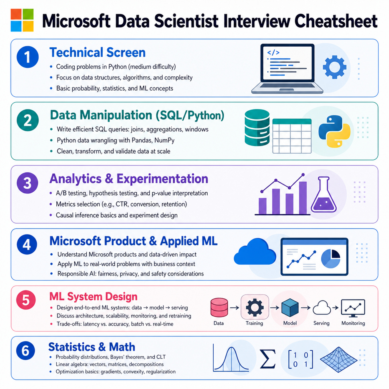
With a 1–2 week timeline, 3/5 ratings across every category, and no solved-question signals, the highest-yield focus is SQL/log queries, A/B testing, and end-to-end ML system design. There are no clear mastered areas from your ratings or activity, so keep deep learning architecture comparisons and behavioral conflict stories as lighter refreshers rather than main study blocks. The Microsoft-specific emphasis is product telemetry, ranking/recommendation evaluation, and responsible-AI production thinking for M365, Azure, and Bing-like products. Budget about 55 minutes for a first-pass cheatsheet review, then spend the rest of your prep time doing timed SQL, experimentation, coding, and ML explanation drills.

Technical Screen — 55 min

Data Manipulation (SQL/Python)

Focus area — Microsoft DS screens lean heavily on SQL; your 3/5 rating and no solved SQL signals make this a high-yield drill.

What's being tested

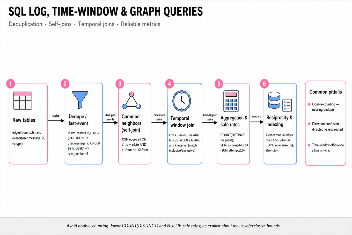
These problems test relational data manipulation skills: deriving graph relationships from directed-edge tables and computing time-windowed event metrics for deliverability. Interviewers probe correct use of joins, window functions, deduplication, temporal joins, and robust aggregation for metric accuracy.

Patterns & templates

• SELF JOIN to find common neighbors: join edges e1 to edges e2 on e1.to = e2.to with e1.from <> e2.from, then GROUP BY and COUNT.

• Use ROW_NUMBER() OVER (PARTITION BY user ORDER BY ts DESC) to deduplicate event streams; filter row_number = 1 for last-event-per-(user,message).

• Temporal joins: inequality join ON a.user=b.user AND b.ts BETWEEN a.ts AND a.ts + interval to capture events in a window; watch inclusive/exclusive bounds.

• Compute rates with safe division: SUM(success) / NULLIF(SUM(attempts),0) to avoid divide-by-zero and report nulls meaningfully.

• Use COUNT(DISTINCT id) when uniqueness matters (unique recipients), otherwise duplicates inflate metrics.

• For mutual edges (friendship), require both (a->b) and (b->a) via self-join and EXISTS or INNER JOIN to enforce reciprocity.

• Index strategy for queries: indexes on (user, ts) and (from, to) speed joins; expect O(n log n) for sorting/window ops, linear for indexed lookups.

Common pitfalls

Pitfall: Double-counting — failing to dedupe message-level events (multiple opens for one message) inflates deliverability rates.

Pitfall: Direction confusion — treating directed edges as undirected when counting common friends yields incorrect reciprocity vs. common-neighbor answers.

Pitfall: Time-window boundaries — mixing inclusive/exclusive intervals or ignoring late-arriving events leads to off-by-one time-window errors.

Practice these the practice cards below cover the canonical variants — solve all of them and time yourself.

Practice questions

Analytics & Experimentation

Focus area — Core DS interview topic; with a 3/5 experimentation rating and no solved evidence, spend extra time on power, MDE, and interpretation.

What's being tested

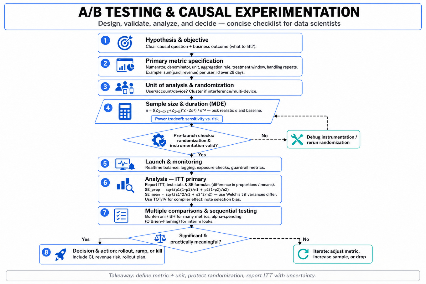
These interviews probe a candidate’s ability to design, analyze, and defend causal experiments end-to-end: picking a precise primary metric, sizing and timing an experiment, choosing randomization and analysis methods that respect the unit-of-analysis, diagnosing instrumentation or randomization failures, and translating statistical lift into product recommendations. Google expects Data Scientists to reason about tradeoffs between sensitivity (power), risk (user and revenue impact), and operational constraints while communicating uncertainty clearly.

Core knowledge

• Unit of analysis: Define the experiment at the correct level (user, account, cookie, device). Mismatch causes biased SEs and misleading p-values; cluster randomization when interference or multi-device users exist.
• Primary metric construction: Precisely specify numerator, denominator, unit, aggregation rule, treatment window, and handling of repeated observations (per-user mean, per-event rate, or sum). Example: primary = sum(paid_revenue) per user_id over 28 days.
• Test statistic & SE formulas: For difference in proportions, use $SE=\sqrt{\frac{p_1(1-p_1)}{n_1}+\frac{p_2(1-p_2)}{n_2}}$; for means, $SE=\sqrt{\frac{s_1^2}{n_1}+\frac{s_2^2}{n_2}}$. Use Welch's t when variances differ.
• Sample size / MDE calc: For two-sided mean test, with equal n: $n=\frac{(Z_{1-\alpha/2}+Z_{1-\beta})^2\cdot 2\sigma^2}{\delta^2}$ where $\delta$ is minimum detectable effect (MDE). Use realistic baseline variance and conversion rates.
• Intent-to-treat (ITT) vs. Treatment-on-treated (TOT): Report ITT as primary; use TOT or instrumental variables to estimate complier effect if noncompliance exists, but note selection bias.
• Covariate adjustment & CUPED: Use pre-period covariates in ANCOVA to reduce variance; CUPED uses a pre-experiment metric to lower $\sigma^2$ and increase power without biasing ITT.
• Multiple comparisons & sequential testing: Control Type I with Bonferroni / BH for many metrics, or use alpha-spending / group-sequential methods (e.g., O’Brien–Fleming) for interim looks; false discovery is common with dashboards.
• Heterogeneous treatment effects: Pre-specify subgroups and interaction tests; beware data-dredging. Use regression with interaction terms for exploratory HTE, and correct for multiplicity when making decisions.
• Duration, ramping, and seasonality: Account for weekdays, marketing events, and user lifecycle. Ensure experiment runs long enough to stabilize metrics (behavioral latency, billing cycles).
• Diagnostics & instrumentation checks: Always run Sample Ratio Mismatch (SRM), unit-consistency tests, pre-period balance, and event-logging completeness. SRM often indicates assignment or logging bugs.
• Non-standard outcomes: For retention or survival outcomes, use Kaplan–Meier and log-rank tests or Cox models for time-to-event; use bootstrap for skewed revenue/LTV.
• Interference & SUTVA violations: If users interact (social features), consider network experiments or cluster/graph-randomization; standard A/B assumptions break otherwise.

Worked example — "Design A/B Test for Subscription Price Increase Effectiveness"

First 30 seconds: clarify the objective (maximize long-run revenue vs. short-term conversion), unit (account or user), and acceptable business constraints (max allowable conversion drop). Pillars of the answer: (1) metric design — primary = 90-day discounted LTV per account_id with secondary metrics conversion_rate and churn; (2) experimental design — randomized rollout at account level, stratify by historical spend or geography; (3) sizing and ramp — compute MDE for revenue per user using baseline mean and variance, plan minimum 8-week run to capture billing cycle; (4) analysis — use ITT for decision-making, regress revenue on treatment with covariate adjustment (ANCOVA), and report bootstrap CI for skewed revenue. Tradeoff to flag: powering for revenue requires large N because variance is high; if business cannot afford long runs, consider powering on conversion (easier) but note mismatch with revenue objective. Close: state guardrails (abort on SRM, large negative churn) and say, "if more time, I'd run a small pilot to validate instrumentation, estimate variance, and consider a price ladder (factorial) to learn elasticity."

A second angle — "Boost Google Workspace Chat Usage with Strategic A/B Testing"

Here the goal is engagement uplift, so metrics and interference look different: primary could be DAU per user or session frequency, and unit is often user_id. Social features create network effects — randomizing at user-level may cause contamination between treated and control (messages cross). You'd consider cluster randomization by team/organization or use exposure modeling. Because engagement changes can be small, use variance reduction (CUPED) and pre-specify subgroup analyses (new users vs. power users). Operationally, real-time metrics and funnel diagnostics matter: if initial increases are from notifications, monitor downstream effects like notification fatigue.

Common pitfalls

Pitfall: Unit-of-analysis mismatch — randomizing on cookie or device while reporting per-user metrics. This underestimates variance and can produce false positives. Always align randomization and analysis unit or use cluster-robust SEs.

Pitfall: Reporting an unanchored metric — saying "lift in conversion = 2%" without stating baseline rate, observation window, or whether it's ITT. Interviewers expect numerator/denominator and CI or p-value.

Pitfall: Ignoring runtime diagnostics and SRM — a statistically significant lift that coincides with a sample-ratio mismatch or logging changes is unreliable. Run SRM, event-completeness, and pre-period balance as part of the analysis pipeline.

Connections

Experimentation work commonly pivots into causal inference on observational data (difference-in-differences, propensity scores) when randomization isn't feasible, or into metric monitoring and anomaly detection to spot experiments that leak. Interviewers may also pivot to ranking/recommender evaluation when experiments affect A/B ranking metrics.

Further reading

• Practical Guide to Controlled Experiments on the Web (Kohavi et al.) — a canonical, practical overview of online A/B testing.
• Evan Miller, A/B Testing: The Complete Guide — hands-on explanations of sample size, sequential testing, and pitfalls.

Practice questions

Microsoft Product & Applied ML

Focus area — Microsoft product teams rely on telemetry; practice defining events, cohorts, tenant/user metrics, retention, and guardrails for M365/Azure-like products.

What's being tested

Interviewers are probing your ability to translate product intent into actionable, testable metrics, choose the correct unit of analysis, and reason about statistical validity and sensitivity. They want to see clear tradeoffs between sensitivity (detecting true product effects) and robustness (avoiding false positives driven by telemetry or segmentation artifacts). At Microsoft scale, emphasis is on reproducible metric definitions, power-aware experiment design, and diagnosing signal vs. noise when telemetry shifts.

Core knowledge

• Unit of analysis: choose between user, user-session, device, or account; inconsistency causes aggregation bias and invalid p-values when intra-unit correlation is large (use ICC to measure).

• Denominator hygiene: define active population precisely (exposure window, eligibility filters), avoid post-randomization filters that induce selection bias; always report numerator, denominator, and inclusion rules.

• Minimum Detectable Effect (MDE) and sample-size formula: for a mean difference, $n = \frac{(Z_{1-\alpha/2}+Z_{1-\beta})^2 \sigma^2}{\Delta^2}$ where $\sigma^2$ is variance of per-unit metric and $\Delta$ is effect size in same units.

• Distributional awareness: use bootstrap or nonparametric tests for heavy-tailed metrics (time-on-task, revenue); aggregate-per-user means reduce variance vs. raw event counts with long tails.

• Guardrail metrics: pre-specify safety metrics (p95 latency, error_rate, DAU) to detect harm; treat them as co-primary or hard-stop depending on business risk.

• Attribution & windows: select conversion/observation windows that match product funnel; shorter windows increase noise, longer windows risk contamination and carryover effects.

• Multiple comparisons & sequential looks: correct via Bonferroni, Benjamini–Hochberg FDR, or alpha-spending (group sequential) rules; uncorrected peeking inflates Type I error.

• Variance reduction: use covariate adjustment (ANCOVA), blocking/stratification by pre-period metric, or CUPED-style techniques to improve power without increasing sample size.

• Metric ownership & computability: ensure the metric is implementable from available telemetry (events, user id, timestamps); specify event-level -> user-level aggregation logic and edge-case handling (duplicates, retries).

• Causal framing & assumptions: randomization must be respected; check for differential attrition, interference (SUTVA violation), and novelty effects. Report ITT and, when appropriate, CACE with instrument strength.

Worked example — "Design an adoption metric and experiment for a new Share button"

First 30 seconds: clarify the goal — is the aim to increase sharing frequency per active user, unique reach, or downstream engagement? Ask about target population, rollout constraints, and guardrails (e.g., performance). Organize the answer around: (1) metric definition, (2) unit and aggregation, (3) experiment design & power, (4) monitoring and guardrails, (5) analysis plan. For the metric pick Shares_per_user_week: count deduplicated share events per user within a 7-day exposure window; define user eligibility and what counts as a share (client event + server confirmation). Choose user as unit; aggregate to per-user means to reduce heavy-tail effects. Power calculation: estimate pre-experiment $\sigma$ from historical per-user share counts, compute sample size for desired MDE. Tradeoff: shorter window improves iteration speed but reduces sensitivity; you’d flag that and propose a parallel longer-window cohort for retention. Close with monitoring plan: pre-specified guardrails (p95 client latency, click_to_share_failure_rate), A/A for randomization checks, and plan for post-hoc segmentation if overall effect is null. If more time: simulate synthetic data to validate power assumptions and plan an uplift model for heterogeneous treatment effects.

A second angle — diagnosing a DAU drop after a rollout

Same core skills apply, but the framing shifts to anomaly diagnosis rather than prospective design. Start with triage: check telemetry for instrumentation changes, evaluate guardrail metrics (error_rate, backend latency), and compare affected cohorts (country, client version). Use decomposition: is drop due to fewer new users (acquisition), lower stickiness (retention), or measurement (missing events)? Run cohort retention curves, segment by adoption day, and compare pre/post per-user event rates. Use statistical control charts and estimate confidence intervals for differences; if randomized rollout existed, use ITT comparisons. Communicate uncertainty and recommend immediate rollback only if guardrails breach pre-specified thresholds.

Common pitfalls

Pitfall: Mixing event-level and user-level inference — testing on raw event counts without adjusting for user-level correlation inflates Type I error; aggregate per unit-of-randomization.

Pitfall: Overfitting to short windows — designing metrics that look good in a 24-hour window but capture novelty, not sustained value; always report multiple windows (short, medium, long).

Pitfall: Ignoring operational definition drift — altering telemetry or deduping rules mid-experiment invalidates comparisons; instead freeze metric code and document versioned definitions.

Connections

Interviewers may pivot to uplift modeling (heterogeneous treatment effects), funnel decomposition and retention modeling, or to experiment platform concerns like randomization fidelity and logging completeness. Be ready to move from metric design to segmentation strategies or to propose diagnostic queries for telemetry sanity checks.

Further reading

• Trustworthy Online Controlled Experiments: A Practical Guide to A/B Testing — Kohavi et al.; covers experiment design, metric choice, and practical pitfalls.

• Evan Miller — A/B Test Sample Size Calculator and Articles — practical tools and clear explanations of MDE, power, and sequential testing considerations.

Practice questions

Focus area — Bing and recommendation surfaces make ranking evaluation useful; add NDCG, MAP, CTR trade-offs, and offline-online metric alignment.

What's being tested

Interviewers assess your ability to design, measure, and interpret ranking and recommendation quality in product settings: choosing appropriate offline proxies, building unbiased online experiments, and diagnosing metric mismatch. Microsoft cares because these systems drive core business outcomes (engagement, retention, revenue) and mistakes in metric definition or experimentation lead to bad launches. Expect to show statistical reasoning, causal thinking, counterfactual evaluation, and tradeoff-aware recommendations rather than engineering or production plumbing.

Core knowledge

• Precision@k / Recall@k / MAP — compute relevance at cutoffs; useful when item relevance labels exist. Precision@k = (# relevant in top-k) / k; stable for small k like 5–10.

• DCG and nDCG — discount by position: $DCG=\sum_{i=1}^k \frac{2^{rel_i}-1}{\log_2(i+1)}$, normalized to ideal DCG to compare queries of different lengths.

• MRR (Mean Reciprocal Rank) — emphasizes first relevant result: $MRR=\frac{1}{N}\sum_{q}\frac{1}{rank_q}$, good for single-goal tasks (e.g., “find answer”).

• Session / downstream metrics — track long-term outcomes like DAU, session length, retention, and conversions; short-term CTR optimization can hurt long-term value.

• Exposure / position bias — clicks are influenced by rank; without correction, offline click labels are biased. Use propensity-weighting or randomized exposure to debias.

• Counterfactual / offline policy evaluation — Inverse Propensity Scoring (IPS): $\hat{V}_{IPS}=\frac{1}{n}\sum_{i}\frac{\pi(a_i|x_i)}{b(a_i|x_i)} r_i$ with high variance when propensities small; prefer Doubly Robust (DR) estimators to reduce variance.

• A/B testing primitives — unit of randomization (user, session, device), sample size and power calculation (detect δ with α, β), and sequential testing corrections (alpha spending, p-value inflation).

• Interference and SUTVA violations — recommendations produce network effects (one user’s exposure affects others); use cluster randomization or reminders that standard A/B assumptions may fail.

• Offline vs online gap diagnosis — log exposures, deterministic seeds, simulate online policy with logged propensities; compare expected engagement (IPS) to observed and inspect distributional shifts (covariate shift, novelty).

• Exploration strategies — epsilon-greedy, Thompson Sampling, and randomized interleaving for online comparison; exploration adds short-term cost but enables unbiased learning/evaluation.

• Business-aligned guardrails — define safety metrics (quality dips, harmful content hits), floor constraints (no negative deltas > X%), and use sequential release (canary, ramp) to limit blast radius.

• Sample size & variance practicalities — for low-base-rate events (rare conversions), need orders of magnitude more traffic; use aggregated metrics, variance reduction (blocking, CUPED), or longer test durations.

Worked example — "Design metrics and experiment to evaluate a ranking change for the Microsoft Store"

First 30s: clarify the unit (user vs session), primary business objective (installs vs revenue vs engagement), and scope (top-k on homepage, personalized vs global). Ask if historical labels exist or only implicit feedback.

Skeleton of an answer:

1. Define primary metric: choose revenue per daily active user if monetization is goal, or session retention at 7 days for long-term engagement; include an immediate proxy like CTR@5 as diagnostic.

2. Offline evaluation: compute nDCG@k and IPS-estimated expected CTR using logged propensities if available; sanity-check with held-out users.

3. Experiment design: randomize at user level, pre-compute power for minimal detectable effect, and plan a staged rollout (20% → 50% → 100%) with guardrail checks.

4. Analysis: use CUPED for variance reduction, check heterogeneity by cohort (new vs returning users), and run sequential checks with alpha spending.

Tradeoff to flag explicitly: optimizing for immediate CTR@5 may reduce discovery and long-term retention; prioritize long-term metric or add an explicit constraint in optimization.

Close: if more time, I'd propose an exploration policy to gather better propensity coverage, a counterfactual DR estimator for offline validation, and a post-hoc causal mediation analysis to see what user behaviors changed.

A second angle — "Offline evaluation for cold-start items and policy comparison"

Same core tools apply but constraints change: very limited historical exposure for new items, so IPS has near-zero denominators and high variance. Instead, propose (1) targeted randomized exposure experiments for cold items to get initial propensities, (2) model-based imputation using content features or collaborative-embedding priors, and (3) offline simulation using a small exploration policy combined with DR estimators. For policy comparison between two rankers, consider interleaving or online interleaving tests to reduce traffic needs and provide direct preference signals. Emphasize the practical balance: you may accept short-term revenue loss to collect unbiased data that enables scalable cold-start evaluation.

Common pitfalls

Pitfall: Optimizing only for clicks. Focusing on CTR alone ignores downstream value; a model that increases clicks but reduces conversion or retention is a failed launch. Always tie to long-term business metrics.

Pitfall: Forgetting to log propensities and exposures. If you don't record the exposure policy probability and ranked-list context, counterfactual estimators are invalid and offline evaluation is biased; plan logging early.

Pitfall: Bad randomization/unit choice. Randomizing at impression-level when users see multiple impressions creates dependence and inflated false positives; prefer user-level or properly clustered randomization and account for interference.

Connections

These topics commonly pivot to causal inference (instrumental variables, mediation), multi-armed bandits / online learning (for exploration-exploitation), and fairness & safety (bias amplification in personalized ranking). Interviewers may probe any of these next.

Further reading

• Practical Guide to Controlled Experiments on the Web — Kohavi et al. — concise best practices for online experiments and guardrails.

• Counterfactual Learning to Rank — Joachims et al. (paper) — foundations for IPS/DR estimators in ranking.

• A Tutorial on Off-Policy Evaluation — Thomas & Brunskill — practical analysis of IPS variance and doubly robust methods.

Practice questions

ML System Design

Statistics & Math

Your stats rating is 3/5 with no metric-practice signals, so keep this as a standard refresher for imbalanced classification.

What's being tested

Candidates must show they can evaluate and compare binary classifiers under realistic constraints: compute and interpret precision–recall curves, choose operating thresholds aligned to asymmetric business costs, and summarize performance with metrics that are meaningful under class imbalance. Interviewers probe statistical correctness (formulas, edge cases), practical computation (sorting, ties, libraries), and how to translate metrics into a decision (threshold choice, expected-cost reasoning) for product or experiment decisions.

Core knowledge

• Confusion matrix entries: true positive (TP), false positive (FP), false negative (FN), true negative (TN); all classification metrics derive from these counts.

• Precision: $\text{Precision} = \frac{TP}{TP+FP}$. Recall (sensitivity): $\text{Recall} = \frac{TP}{TP+FN}$. F1: harmonic mean $2\frac{P\cdot R}{P+R}$.

• Precision–recall curve: plot precision (y) vs recall (x) by sweeping the threshold on model scores; points correspond to unique score cutoffs after sorting predictions by descending score.

• Average Precision (AP) / AUPRC: area under the precision–recall curve; AP emphasizes performance on the positive class—baseline equals positive prevalence ($\pi = \frac{P}{N}$), so AUPRC > $\pi$ is meaningful.

• Why prefer PR over ROC: ROC/AUROC can be overly optimistic on rare positives because false positive rate uses TN in denominator; PR focuses on positives and is sensitive to class imbalance (see Saito & Rehmsmeier).

• Computation details: sort by score $O(n\log n)$, compute cumulative TP/FP in one pass $O(n)$, handle ties by grouping equal-score records or using rank-average; Python libraries (scikit-learn precision_recall_curve, average_precision_score) implement standard variants.

• Edge cases: no positives $\Rightarrow$ recall undefined (or zero) and baseline AP = 0; no negatives leads to precision = 1 at all recalls; report these explicitly when presenting results.

• Threshold selection under asymmetric costs: minimize expected cost $E[C]=c_{FN}\cdot FN + c_{FP}\cdot FP$ or equivalently choose threshold where likelihood ratio $\frac{p(y=1|x)}{p(y=0|x)}$ exceeds cost ratio; calibration of probabilities matters for cost-based thresholds.

• Reporting: show the full PR curve, AP value, and one or two operating points (threshold, confusion matrix, precision/recall) with business-aligned cost interpretation and confidence intervals (bootstrap).

• Statistical uncertainty: obtain CI on AP/precision/recall via bootstrap or stratified resampling; for small positive counts use exact binomial intervals for recall at a point.

• Ranking vs probability: PR curve works with ranked scores; if scores are uncalibrated, ranking-based metrics (AP) still valid, but cost-minimizing thresholds require calibrated probabilities (Platt scaling, isotonic regression).

• Visualization nuance: PR curves are often step functions; interpolation method (interpolating precision at increased recall) affects AP numeric value—state which method used.

Worked example — Compute and plot a precision–recall curve

Frame: ask whether you have probabilistic scores or only binary predictions, confirm the evaluation set is holdout and whether positives are rare or sample-weighted. Skeleton: (1) sort predictions by descending score, (2) sweep unique thresholds computing cumulative TP/FP to get precision and recall points, (3) plot precision vs recall and compute Average Precision with trapezoidal/integration rule, (4) annotate business-relevant operating points and CI via bootstrap. Tradeoff to call out: whether to group ties (same-score examples) — grouping yields fewer thresholds and a stable curve, but may slightly change AP; document your tie strategy. If using scikit-learn, call precision_recall_curve and average_precision_score and state which interpolation they implement. Close: say you'd next derive threshold(s) that minimize expected cost using calibrated probabilities and produce bootstrap CIs for AP and for the chosen operating point.

A second angle — Choose Classification Metrics Under Asymmetric Costs

Here the same precision/recall machinery informs a cost-sensitive decision. Start by eliciting business costs: quantify $c_{FP}$ and $c_{FN}$ or their ratio. Convert costs to an objective: choose the threshold that minimizes $E[C]=c_{FN}\cdot FN + c_{FP}\cdot FP$ on validation data (or expected over calibrated probabilities). Present both a visual approach (overlay cost lines on PR or ROC space) and a numeric one (compute cost at each threshold).

Tip: Flag calibration: if model scores are poorly calibrated, map scores to calibrated probabilities before computing expected cost; otherwise thresholding by raw score may be suboptimal.

For extremely imbalanced positives, consider decision rule based on top-K predictions if downstream capacity or attention is limited.

Common pitfalls

Pitfall: Reporting accuracy as the main metric on imbalanced data. Accuracy can be near 100% with a useless model; prefer PR/AUPRC and confusion-matrix at selected thresholds.

Pitfall: Treating AUROC and AUPRC as interchangeable. AUROC measures separability across both classes; AUPRC focuses on positive-class retrieval and is sensitive to prevalence—use AUPRC for rare positives.

Pitfall: Selecting thresholds without accounting for probability calibration. If you optimize expected-cost on uncalibrated scores, your chosen threshold and estimated costs will be biased; calibrate (e.g., Platt scaling) or use ranking-based objectives if calibration isn't possible.

Connections

Precision–recall analysis frequently connects to probability calibration, cost-sensitive learning (cost matrices, asymmetric loss), and ranking metrics (AP, nDCG) for top-K decisions. Interviewers may pivot to model calibration methods, uplift/causal metrics for treatment targeting, or experiment-design consequences of classifier thresholds.

Further reading

• scikit-learn precision-recall documentation — implementation notes and function behavior for precision_recall_curve and average_precision_score.

• Saito & Rehmsmeier (2015), “The precision‑recall plot is more informative than the ROC plot when evaluating binary classifiers on imbalanced datasets” — explains when and why to prefer PR curves.

Practice questions

Machine Learning

You viewed ML content but have no solved signal; refresh tuning, scaling, PCA, and K-Means trade-offs.

What's being tested

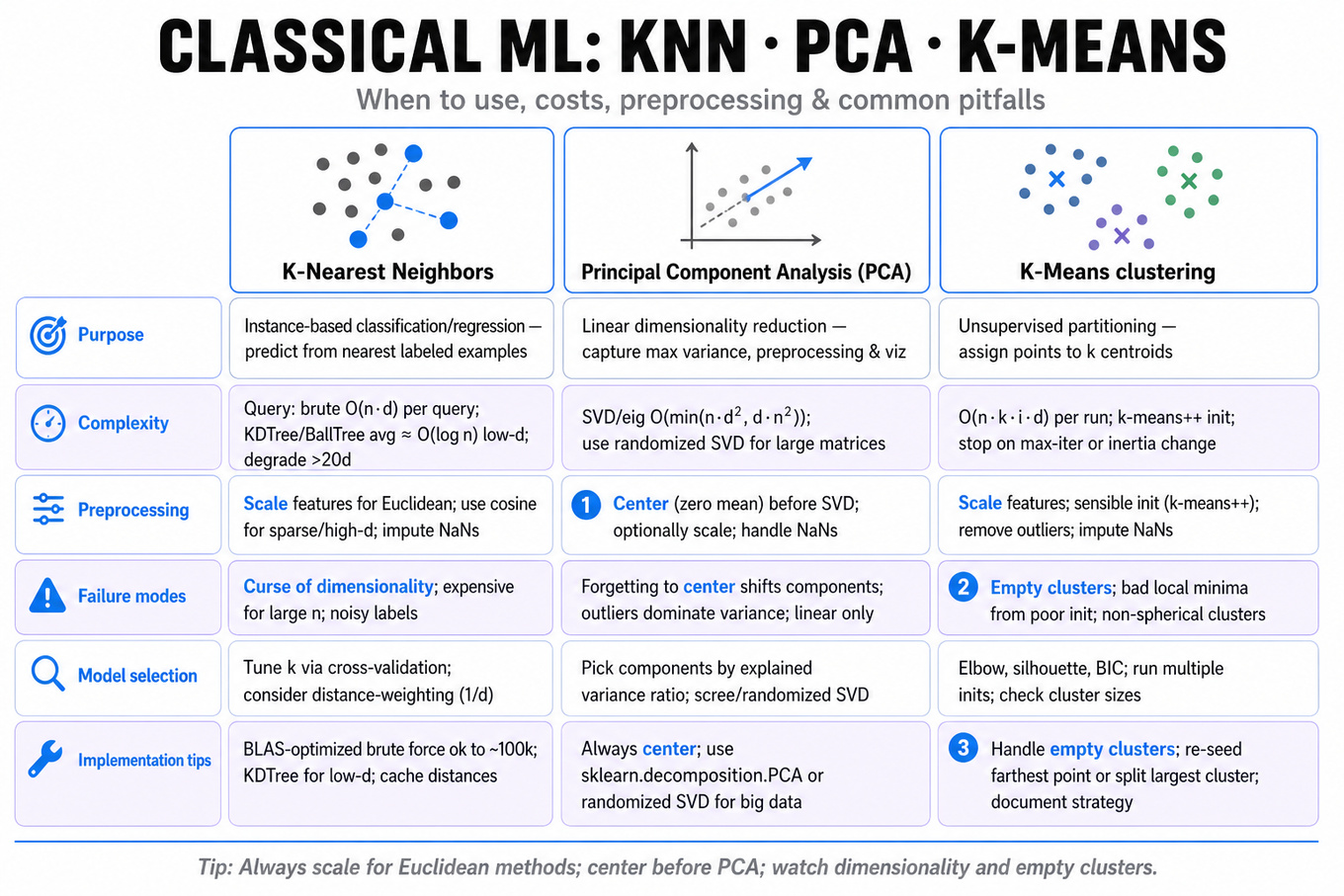
These questions test practical mastery of K-Nearest Neighbors, Principal Component Analysis, and K-Means: algorithmic behavior, preprocessing effects, numerical/implementation robustness, and hyperparameter selection. Interviewers want a Data Scientist who can choose the right tradeoffs (accuracy vs. scalability), diagnose failure modes (high-dimensional data, empty clusters), and implement/validate clustering and instance-based models reliably.

Patterns & templates

• Brute-force KNN: compute pairwise distances O(n·d) per query, then sort/select k; acceptable for n up to ~100k with optimized BLAS, else use indices.

• Indexed KNN: use `KDTree`/`BallTree` for low-dimensional data (average query ≈ O(log n)); deteriorates under the curse of dimensionality.

• Distance choices: pick Euclidean for continuous features, cosine for sparse/high-d vectors, and consider distance-weighting (1/d) for soft voting.

• PCA workflow: center data, compute SVD or eigendecomposition (`sklearn.decomposition.PCA`); complexity ≈ O(min(n·d^2, d·n^2)); use randomized SVD for large matrices.

• K-Means basics: Lloyd’s algorithm with `k-means++` init (`sklearn.cluster.KMeans`), complexity O(n·k·i·d); stop on max-iter or small inertia change.

• Empty-cluster handling: re-seed from farthest point, split largest cluster, or reduce k; document chosen strategy.

• Model selection: tune k via cross-validation for KNN, elbow/silhouette/BIC for K-Means, and explained variance ratio for PCA components.

• Scaling & preprocessing: always scale features for Euclidean-based methods; impute or drop NaNs; consider PCA before KNN in very high-d sparse data.

Common pitfalls

Pitfall: Treating `KDTree` as a cure-all—trees often perform worse than brute force in >20 dimensional data.

Pitfall: Forgetting to center data before PCA, which shifts principal components and invalidates explained variance.

Pitfall: Ignoring empty clusters in K-Means implementations; silent failures produce biased centroids and wrong cluster counts.

Practice these

The practice cards below cover the canonical variants — solve all of them and time yourself.

Practice questions

Behavioral & Leadership

Microsoft values cross-functional ownership; rehearse one product-impact story tied to measurable KPIs and trade-offs.

What's being tested

Interviewers are probing a candidate's ability to lead an ambiguous ML project end-to-end while staying metric-driven, pragmatic, and communicative. Expect evaluation of problem framing into measurable business KPIs, experimental and causal reasoning, trade-off articulation (e.g., short-term lift vs. long-term health), and stakeholder alignment under uncertainty. The interviewer wants evidence you can turn fuzzy goals into defensible analysis, iterate with experiments, and quantify outcomes so decisions are data-grounded.

Core knowledge

• Problem framing → metric tree: translate product goals into one primary North Star metric and 1–3 guardrail metrics (e.g., increase DAU while keeping CTR and retention stable), document assumptions and expected causal path.

• Causal vs observational: know when an effect requires an A/B test versus when observational techniques (adjustment, propensity score) or quasi-experimental designs (difference-in-differences) are appropriate.

• Statistical power & sample-size: compute required sample using the classic two-proportion formula; e.g. $n\approx\frac{(Z_{1-\alpha/2}+Z_{1-\beta})^2\left[p_1(1-p_1)+p_2(1-p_2)\right]}{(p_1-p_2)^2}$ and trade off detectable effect vs time-to-result.

• Metric design & leakage: define denominator and unit of analysis (user, session, query) to avoid Simpson’s paradox and metric leakage from downstream signals; prefer pre-aggregated, raw event signals for primary metrics.

• Multiple comparisons & sequential testing: adjust for peeking with alpha spending or Bonferroni/BH corrections; for continuous rollout prefer sequential or platform-implemented stopping rules.

• Model evaluation vs product impact: tie offline metrics (AUC, RMSE) to expected online impact; compute expected value lift (e.g., precision@k → incremental conversions) and simulate decision thresholds using expected utility.

• Bias, confounding, and DAGs: draw a causal DAG to spot back-door paths and colliders; apply back-door adjustment or instrumental variable if needed.

• Robustness & sensitivity: run subgroup, time-window, and placebo checks; report effect heterogeneity and worst-case sensitivity bounds (e.g., Rosenbaum-style).

• Deployment & monitoring metrics: specify post-launch SLOs for model performance (e.g., calibration drift, delta in primary metric), data freshness checks, and rollback criteria tied to measurable thresholds.

• Stakeholder & trade-off communication: prepare three artifacts: 1) concise one-pager with KPI, success criteria, timeline; 2) prioritized data gaps and required experiments; 3) plan for interpretation and next steps if results are ambiguous.

Worked example — Describe leading an ambiguous ML project end-to-end

Start by clarifying the business goal in 2–3 quick questions: "What's the exact business KPI (monetary or engagement) and the acceptable trade-offs/guardrails?" State assumptions (unit of analysis = user-week; success = +2% lift in metric within 8 weeks). Organize the answer into four pillars: (1) Define outcome metric, unit, and causal hypothesis with a simple DAG; (2) Assess available signals and data quality—identify missing covariates and privacy constraints; (3) Experiment & model: choose between direct A/B test of model-backed feature vs offline uplift modeling, describe evaluation (power calc and holdout period); (4) Launch & monitor: rollout plan with canary, metrics to watch, and rollback thresholds. Flag a tradeoff: optimizing for short-term conversion may harm long-term retention—propose multi-objective evaluation or constrained optimization. Close with "if I had more time" items: deeper causal analysis (instrumental variables or longer-term cohort study), and an uplift experiment to measure heterogeneous treatment effects.

A second angle — Resolve conflict with measurable outcome

In a stakeholder conflict (product wants fast rollout; legal wants privacy-first), reframe the dispute into measurable criteria: quantify potential benefit, privacy risk, and worst-case cost. Propose a staged path: run a privacy-preserving pilot (e.g., aggregated signals, differential privacy parameter tuned) with a strict p-value/effect-size threshold for expansion. Use neutral metrics (business uplift, false-positive rate, privacy leakage score) so decisions map to numbers, not opinions. Emphasize negotiated guardrails up front and document the decision rule that converts metric results into action.

Common pitfalls

Pitfall: Mistaking correlation for causation — describing observational uplift and claiming causal impact without randomization or valid adjustment undermines credibility. Always state identification assumptions and preferred experimental design.

Pitfall: Overfocusing on offline model metrics — citing only AUC or loss without mapping to product impact (value-per-action, cost-per-conversion) makes recommendations un-actionable. Translate offline gains to expected business units.

Pitfall: Poor stakeholder alignment — failing to agree on success criteria and timelines leads to scope drift. Start by writing the one-pager and confirm sign-off before heavy analysis.

Connections

Interviewers may pivot to experiment platform design (metrics pipelines, segmentation), causal inference methods (instrumental variables, synthetic controls), or model governance (fairness, privacy constraints like differential privacy) — be ready to link your decisions to these adjacent areas without owning their implementation.

Further reading

• Trustworthy Online Controlled Experiments: A Practical Guide to A/B Testing — a practical playbook for experiment design and pitfalls (Kohavi-style guidance).

• Causal Inference in Statistics: A Primer — accessible overview of identification, back-door, and instrumental variable strategies.

Practice questions