Amazon Data Scientist Interview Prep Guide

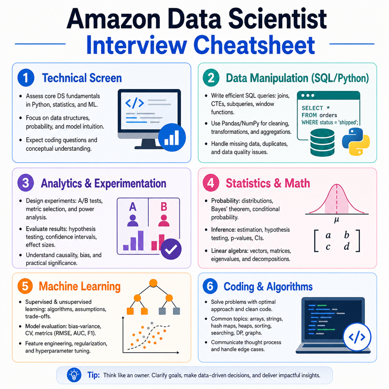
Your biggest focus is rebuilding fundamentals from first principles: statistics/probability, ML evaluation, SQL/Pandas edge cases, algorithms, and especially metrics design because you noted you’re coming from academia and weak on industry metric framing. You’re comparatively more comfortable with core SQL and some causal-inference framing, so those stay lighter than the many “new” ML, coding, window-function, timezone, and ETL subtopics you flagged. For Amazon, this plan highlights customer/backward-working metrics, experiment guardrails, marketplace-style root-cause analysis, production data reliability, recommender/forecasting systems, and Leadership Principle STAR stories. Because your timeline is still exploratory, use this as a foundation-building plan rather than a cram plan: prioritize emphasized concepts first, then cycle through normal concepts for breadth.

Technical Screen — 69 min

Data Manipulation (SQL/Python)

• SQL Analytical Querying And Data Modeling (Focus) — covered in depth under Onsite below.

• Python/Pandas Data Manipulation (Focus) — covered in depth under Onsite below.

• Data Pipeline Reliability And Stream Processing (Focus) — covered in depth under Onsite below.

Analytics & Experimentation

• A/B Testing And Statistical Inference (Focus) — covered in depth under Onsite below.

• Product Metrics, Root-Cause Analysis And Visualization (Focus) — covered in depth under Onsite below.

Statistics & Math

• Probability, Conditional Expectation And Bayes Rule (Focus) — covered in depth under Onsite below.

• Linear Regression, OLS Diagnostics And Assumptions (Focus) — covered in depth under Onsite below.

Machine Learning

• Supervised ML Fundamentals, Evaluation And Feature Engineering (Focus) — covered in depth under Onsite below.

• ML System Design, Recommenders, Forecasting And Allocation (Focus) — covered in depth under Onsite below.

Coding & Algorithms

• Coding Algorithms And Data Structures (Focus) — covered in depth under Onsite below.

Onsite — 69 min

Data Manipulation (SQL/Python)

Focus area — Core SQL was rated solid, but you flagged many new SQL subtopics: windows, null joins, top-N, cohorts, FX, and intervals.

What's being tested

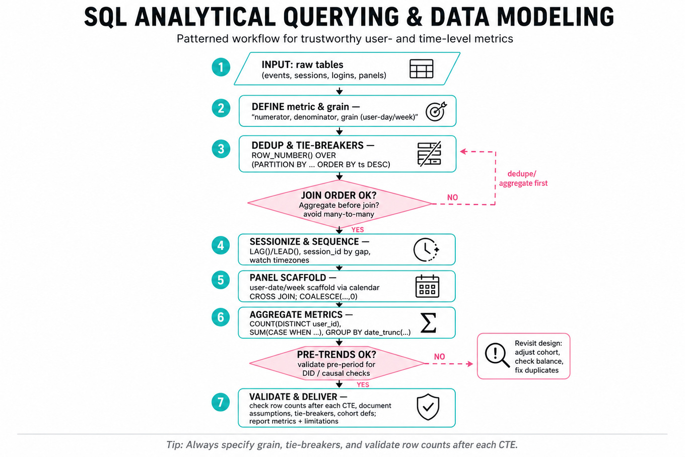
You’re being tested on analytical SQL for product and causal analysis: converting raw event, login, session, and panel tables into trustworthy user-level or time-level metrics. Interviewers look for clean use of joins, deduplication, window functions, temporal logic, and aggregation that supports Data Scientist decisions, not data-pipeline design.

Patterns & templates

• User/event aggregation with COUNT(DISTINCT user_id), SUM(CASE WHEN...), and GROUP BY date_trunc(...); define numerator, denominator, and grain first.

• Window functions like ROW_NUMBER(), LAG(), LEAD(), and RANK() OVER (PARTITION BY ... ORDER BY ...); always specify tie-breakers.

• Session and event sequencing by timestamp using LAG(event_ts) or LEAD(event_ts); watch time zones, missing events, and duplicate logs.

• Panel construction via user-date or user-week scaffolds using CROSS JOIN calendar tables; fill missing periods with COALESCE(..., 0).

• Causal-analysis prep for DID: create treated, post, and interaction terms; estimate effect as $(\Delta treated) - (\Delta control)$ after validating pre-trends.

• Cross-channel attribution using conditional distinct counts and set logic; decide whether users can belong to multiple channels or require mutually exclusive assignment.

• Efficient large-table SQL: filter early with WHERE, aggregate before joining, avoid accidental many-to-many joins, and inspect row counts after each CTE.

Common pitfalls

Pitfall: Counting events instead of users. If the metric is user proportion, use COUNT(DISTINCT user_id), not raw login rows.

Pitfall: Joining before deduplicating. A many-to-many join can silently inflate engagement, hours, or treatment effects.

Pitfall: Treating SQL output as final analysis. For DS work, explain assumptions, metric grain, cohort definitions, and validation checks.

Practice these

The practice cards below cover the canonical variants — solve all of them and time yourself.

Practice questions

Focus area — You rated Pandas shaky and selected rolling windows, timezone-aware dates, retention, deduplication, and historical conversions for extra practice.

What's being tested

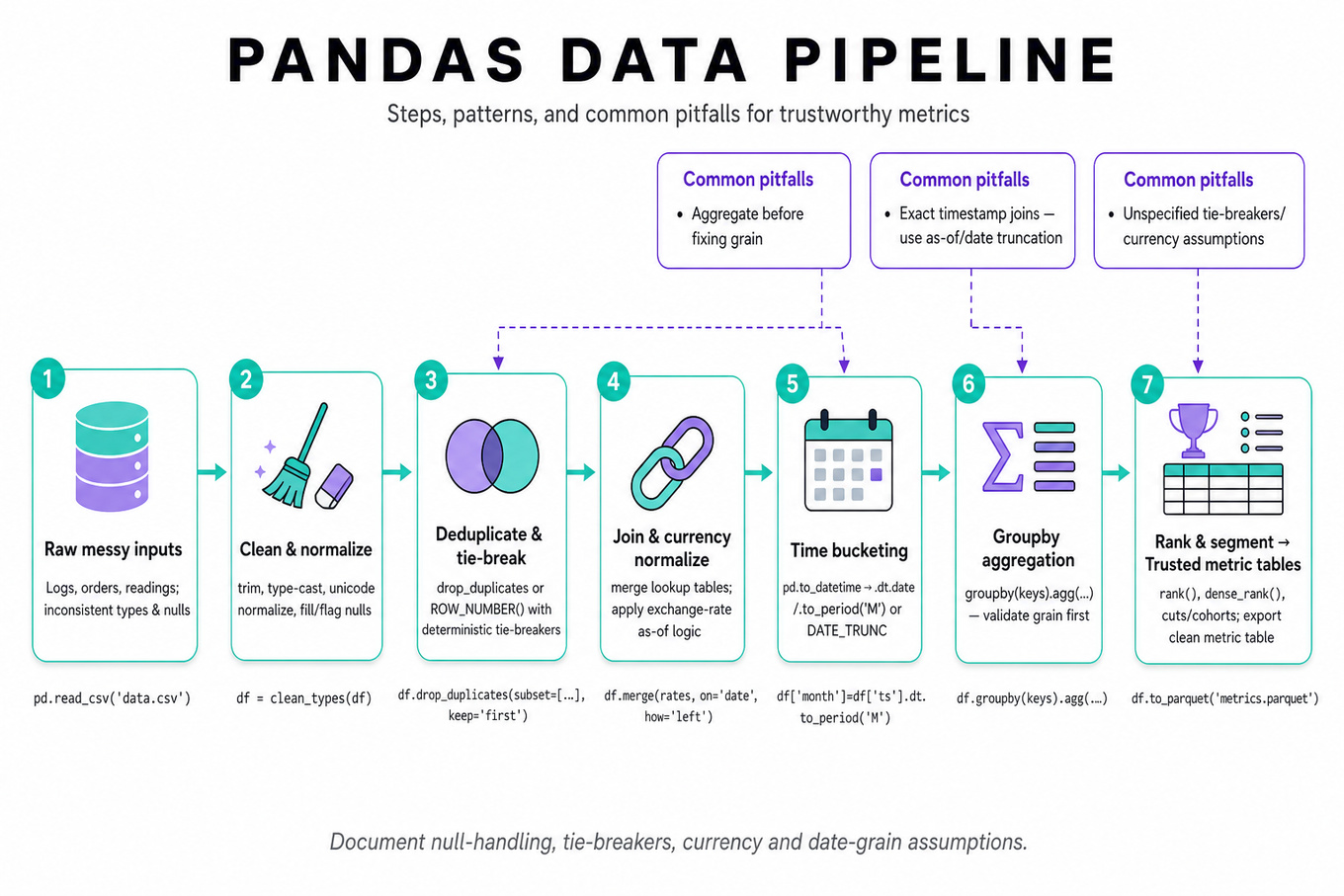
This tests analysis-grade data manipulation in pandas and SQL: cleaning messy inputs, joining heterogeneous tables, aggregating by time/customer/product segments, and ranking or deduplicating records correctly. Interviewers are probing whether you can produce trustworthy metric tables under realistic ambiguity: duplicate events, currency normalization, date granularity, missing values, and tie-breaking.

Patterns & templates

• Groupby aggregation in pandas: df.groupby(keys).agg(...) for revenue, counts, kWh, or sales totals; validate row grain before aggregating.

• Time bucketing with pd.to_datetime, .dt.date, .dt.to_period("M"), or SQL DATE_TRUNC; avoid mixing timestamps and dates accidentally.

• Deduplication by business key using drop_duplicates(subset=..., keep=...) or ROW_NUMBER() OVER (...); declare deterministic tie-breakers.

• Join then normalize pattern: merge facts to lookup tables like exchange rates using merge; check many-to-one assumptions before computing converted metrics.

• Ranking within groups via rank, sort_values, cumcount, or SQL DENSE_RANK; specify whether ties should share rank.

• Conditional segmentation using np.where, pd.cut, CASE WHEN, and boolean masks for Prime/non-Prime, price buckets, or customer cohorts.

• Streaming/counting basics for text-like inputs: use collections.Counter or plain dict; Unicode normalization with unicodedata.normalize and regex tokenization.

Common pitfalls

Pitfall: Aggregating before fixing grain. If order lines are duplicated or salaries repeat by country/date, totals and ranks become silently wrong.

Pitfall: Treating date joins as exact timestamp joins. Exchange rates, sales days, and meter readings often require explicit date extraction or as-of logic.

Pitfall: Returning code without explaining assumptions. Say how you handle nulls, duplicates, ties, currencies, and timezone/date boundaries.

Practice these

The practice cards below cover the canonical variants — solve all of them and time yourself.

Practice questions

Focus area — You marked idempotent ETL, upserts, CDC ordering, exactly-once semantics, and staging swaps as new, so reliability needs first-principles coverage.

What's being tested

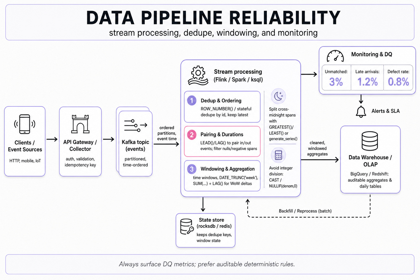
These problems test practical SQL/Python data-manipulation skills: joining event and reference tables, computing per-entity metrics, and using window functions to handle ordering, deduplication and week-over-week changes. Interviewers probe whether you can produce correct, auditable metrics from messy time-series data and explain tradeoffs for edge cases.

Patterns & templates

• ROW_NUMBER() over partitions for deduping: ROW_NUMBER() OVER (PARTITION BY id ORDER BY ts DESC) to keep the latest record.

• Pair in/out events with LEAD()/LAG() — compute durations as lead(ts)-ts, filter nulls and negative spans.

• Split cross-midnight shifts by truncating and using GREATEST()/LEAST() or generate_series() for per-day allocation.

• Aggregate defects: SUM(CASE WHEN condition THEN 1 ELSE 0 END) and defect rate = defects/NULLIF(total,0).

• Week-over-week: use DATE_TRUNC('week', dt) then SUM(...) + LAG() window to compute changes and percent deltas.

• Use GROUP BY + ORDER BY with ROW_NUMBER() to extract top-N lanes/carriers per metric; tie-break on stable key (e.g., carrier_id).

Common pitfalls

Pitfall: Pairing events by simple self-join without ordering — leads to wrong durations when multiple ins or outs exist. Always order and dedupe first.

Pitfall: Dividing by zero or using integer division — wrap denominators with NULLIF and cast to numeric to avoid truncation.

Pitfall: Ignoring late-arriving or duplicate events — surface a data-quality metric (e.g., percent unmatched events) instead of assuming perfect data.

Practice these

the practice cards below cover the canonical variants — solve all of them and time yourself

Practice questions

Analytics & Experimentation

Focus area — Statistics is 1/5, CI and power topics are shaky, and Amazon DS screens frequently probe experiments, guardrails, and decision rules.

What's being tested

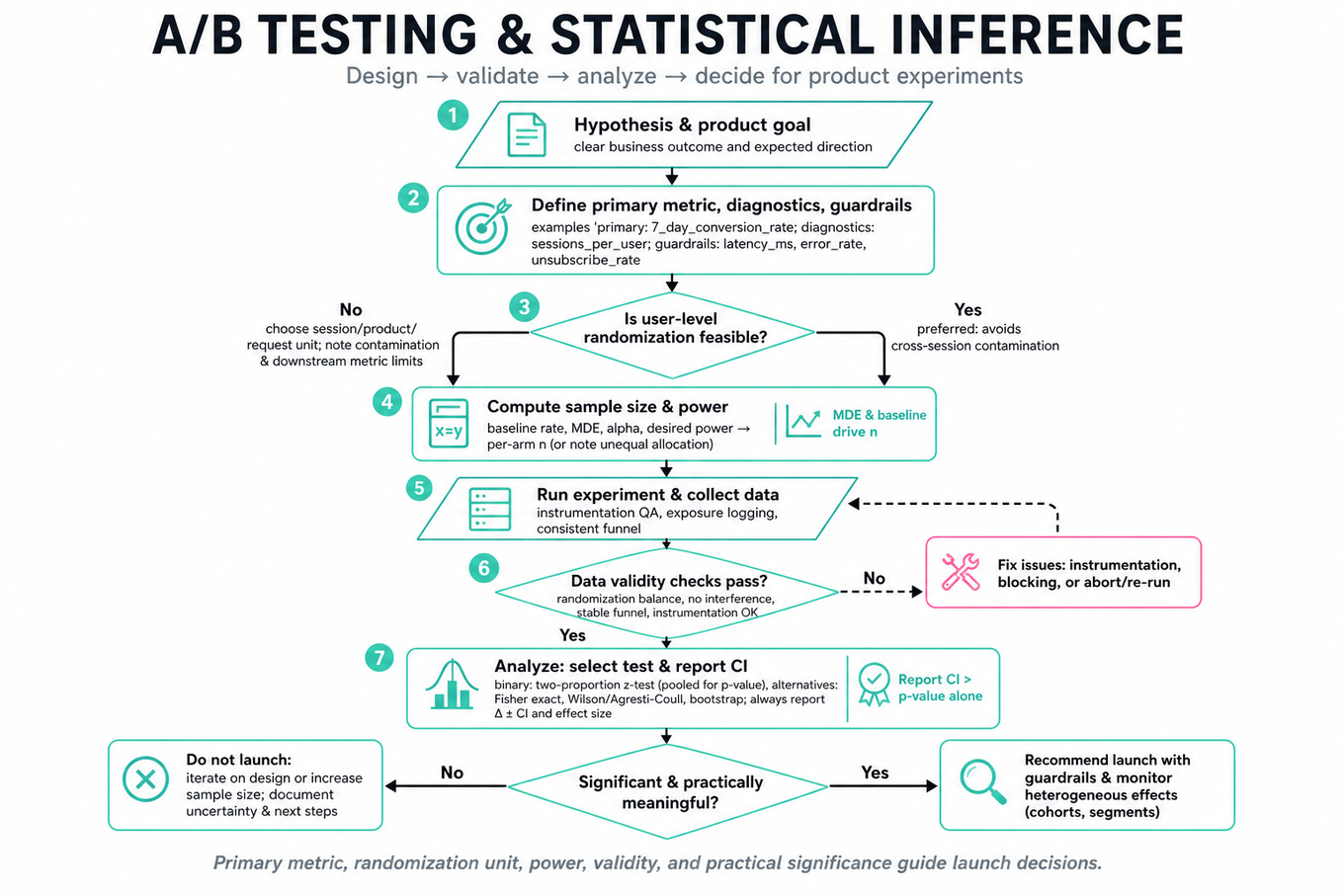
Interviewers are probing whether you can design, analyze, and explain online controlled experiments as a Data Scientist, not just run a canned significance test. You need to connect business/product goals to measurable outcomes, choose the right statistical test, check experiment validity, and make a launch recommendation under uncertainty. Amazon cares because small product changes at scale can move conversion_rate, CTR, revenue_per_visitor, delivery promises, or customer trust metrics, and a misleading experiment can cause expensive false launches or missed opportunities. Expect the interviewer to test both mechanics—sample size, confidence intervals, p-values—and judgment: metric selection, guardrails, heterogeneous effects, multiple comparisons, and whether the result is practically meaningful.

Core knowledge

• Randomized controlled trials estimate causal impact by assigning users, sessions, products, or requests to treatment and control before exposure. For most product experiments, user-level randomization is preferred because it avoids cross-session contamination and supports customer-level metrics like 7_day_conversion_rate.

• Metric design starts with a primary success metric, secondary diagnostic metrics, and guardrail metrics. Example: for a dashboard engagement test, primary could be weekly_active_users, secondary could be dashboard_sessions_per_user, and guardrails could include latency_ms, error_rate, unsubscribes, or downstream purchase_rate.

• Two-proportion z-tests are common for binary outcomes. For control conversion $\hat p_c=x_c/n_c$ and treatment conversion $\hat p_t=x_t/n_t$, the difference is $\Delta=\hat p_t-\hat p_c$. Under the null, use pooled rate $\hat p=(x_t+x_c)/(n_t+n_c)$ and standard error $SE_0=\sqrt{\hat p(1-\hat p)(1/n_t+1/n_c)}.$ Then $z=\Delta/SE_0$.

• Confidence intervals communicate estimation uncertainty better than p-values alone. For a binary metric difference, a common large-sample CI is $\Delta \pm z_{1-\alpha/2}\sqrt{\frac{\hat p_t(1-\hat p_t)}{n_t}+\frac{\hat p_c(1-\hat p_c)}{n_c}}.$ For small counts or rare events, mention Wilson, Agresti-Coull, Fisher’s exact test, or bootstrap as more robust alternatives.

• Power and sample size depend on baseline rate, minimum detectable effect, significance level, and desired power. For equal-sized two-arm binary tests, approximate per-arm sample size is $n \approx \frac{2\bar p(1-\bar p)(z_{1-\alpha/2}+z_{1-\beta})^2}{\delta^2},$ where $\delta$ is the absolute effect size. Smaller detectable effects require quadratically larger samples.

• Practical significance is different from statistical significance. At Amazon scale, a 0.03 percentage-point lift may be statistically significant but not worth shipping if it adds operational complexity, harms latency, or degrades a long-term trust metric. Always translate effect size into business/customer impact.

• Sample ratio mismatch is a validity check before interpreting treatment effects. If a planned 50/50 split produces 41/59 users, run a chi-square check against expected assignment counts. SRM often indicates assignment bugs, logging gaps, bot filtering asymmetry, eligibility mistakes, or exposure leakage.

• Unit of analysis must match the randomization unit. If randomization is by user but analysis treats page views as independent, p-values will be too small because within-user observations are correlated. Aggregate to user-level metrics or use cluster-robust standard errors when outcomes are repeated or clustered.

• Multiple testing inflates false positives when checking many metrics, segments, or variants. Bonferroni controls family-wise error with $\alpha/m$ but can be conservative; Benjamini-Hochberg controls false discovery rate. For interviews, say which comparisons were pre-registered versus exploratory.

• Variance reduction improves sensitivity without increasing traffic. CUPED uses pre-experiment behavior as a covariate: $Y_{adj}=Y-\theta(X-\bar X)$, where $X$ is a pre-period metric correlated with the outcome. It is especially useful for noisy continuous metrics like spend, sessions, or engagement time.

• Heterogeneous treatment effects should be handled carefully. Segment analysis by device, geography, new vs returning users, Prime vs non-Prime, or traffic source can reveal important effects, but these cuts are usually underpowered and subject to multiple comparison risk. Treat them as diagnostics unless pre-specified.

• Experiment duration should cover business cycles and avoid peeking-driven decisions. A 7-day test captures weekday/weekend behavior, but seasonality, promotions, novelty effects, and delayed conversions may require longer windows. If monitoring continuously, use sequential testing or alpha-spending rather than repeatedly checking naive p-values.

Worked example

For “Analyze an A/B test over last 7 days”, a strong candidate should start by clarifying the randomization unit, intended traffic split, eligibility criteria, primary metric, and whether the 7-day window is complete for delayed outcomes. Then state assumptions: users were randomized before exposure, assignment was stable, and each user is counted once for the primary binary conversion metric. The answer can be organized into four pillars: first, validate the experiment with sample sizes, exposure counts, and sample-ratio mismatch; second, compute treatment and control conversion rates plus absolute and relative lift; third, run statistical inference using a two-proportion z-test and confidence interval; fourth, inspect guardrails and important segments.

A good candidate would explicitly say they would not jump straight to “p < 0.05, ship it” before checking data validity and practical impact. For example, if treatment improves conversion_rate but worsens refund_rate, latency_ms, or customer complaints, the launch recommendation may change. One tradeoff to flag is whether to use all events or user-level aggregation: event-level analysis gives more rows but violates independence if the user is the randomized unit. The candidate should close with a decision framework: launch if the primary metric lift is statistically and practically meaningful, guardrails are neutral, SRM is clean, and effects are directionally consistent across major cohorts. If given more time, they should mention checking novelty effects, delayed conversions, pre-period balance, and whether the result holds under variance-reduced or cluster-robust analysis.

A second angle

For “Calculate A/B sample size, CI, decision rules”, the same ideas appear before the experiment rather than after it. The interviewer is testing whether you can design a test with enough power to detect a business-relevant effect, not reverse-engineer significance once the data arrives. You should ask for baseline conversion rate, minimum detectable effect, desired power, alpha, number of variants, and whether the metric is binary, continuous, ratio-based, or clustered. The framing shifts from “what happened?” to “what evidence will we require to make a decision?” A strong answer includes an explicit decision rule, such as: launch only if the 95% CI excludes zero, the lower bound exceeds the practical threshold, and guardrails remain within acceptable limits.

Common pitfalls

Pitfall: Treating p-value as the probability the null hypothesis is true.

A p-value is the probability of observing data at least as extreme as this result assuming the null is true. It is not $P(H_0 \mid data)$, and it does not measure effect size. A stronger answer pairs the p-value with a confidence interval, absolute lift, relative lift, and business impact.

Pitfall: Ignoring experiment validity checks and going straight to inference.

A tempting but weak answer is: “Control converted at 10%, treatment at 11%, p < 0.05, so ship.” Better: first check assignment ratio, exposure logging, duplicate users, bot/internal traffic, pre-period balance, metric denominator consistency, and whether the analysis unit matches randomization. Invalid randomization can make a beautiful confidence interval meaningless.

Pitfall: Overfitting the narrative to segments.

Candidates often slice by country, browser, customer tenure, and device until they find one impressive subgroup. That is exploratory analysis and should be labeled as such. The stronger version is to pre-specify key segments, correct or caveat multiple testing, and recommend follow-up experiments for surprising heterogeneous effects.

Connections

Interviewers may pivot from here to causal inference for non-randomized launches, including difference-in-differences, matching, regression adjustment, or instrumental variables. They may also connect to metric design, ranking/recommender evaluation, sequential testing, CUPED, or anomaly diagnosis when an experiment result conflicts with dashboard trends.

Further reading

• Trustworthy Online Controlled Experiments by Kohavi, Tang, and Xu — Practical treatment of experiment design, validity threats, metrics, and decision-making in large-scale online platforms.

• Controlled experiments on the web: survey and practical guide, Kohavi et al. — Seminal paper on online A/B testing pitfalls, ramping, metrics, and organizational practice.

• Improving the Sensitivity of Online Controlled Experiments by Deng, Xu, Kohavi, and Walker — Introduces CUPED-style variance reduction for online experiments.

Practice questions

Focus area — You specifically noted an academic background and weak metrics design, so Amazon-style customer, Prime, funnel, and marketplace metrics get extra space.

What's being tested

Interviewers are probing whether you can turn ambiguous business movement into trustworthy metrics, diagnostic cuts, and clear visual evidence without over-claiming causality. For Amazon Data Scientists, this matters because decisions often depend on operational dashboards, funnel metrics, marketplace balance, recommender quality, or customer experience signals where a small metric shift can represent millions of dollars or degraded customer trust. You are expected to know how visualization tools like `Tableau` affect metric interpretation, but from an analysis layer: joins, filters, level of detail, aggregation grain, and dashboard usability. The strongest answers combine product intuition, statistical discipline, and practical dashboard design: define the metric, validate it, segment it, visualize it, and state what evidence would change your conclusion.

Core knowledge

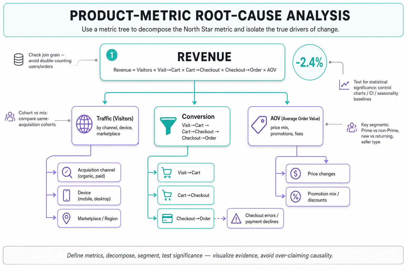
• Metric definition comes before visualization. For any decline or dashboard, define numerator, denominator, entity grain, time window, inclusion/exclusion rules, and refresh cadence. For example, `conversion_rate` = orders / sessions differs materially from `buyer_conversion` = buyers / visitors.

• Metric decomposition is the core root-cause tool. Break aggregate movement into components:
  $\Delta Revenue \approx \Delta Traffic \times Conversion \times AOV$
  More explicitly: `Revenue` = Visitors × Visit-to-Cart × Cart-to-Checkout × Checkout-to-Order × AOV.

• Segmentation should test plausible mechanisms, not create random slices. Common Amazon-relevant cuts include marketplace, device, acquisition channel, Prime status, new vs returning customers, category, fulfillment speed, seller type, inventory availability, and recommendation surface.

• Cohort analysis separates mix shifts from behavior changes. Compare users acquired in the same period or exposed to the same experience, then track retention, repeat purchase, defect rate, or revenue over age. This prevents confusing “more new users” with “worse engagement.”

• Statistical noise matters in root-cause diagnosis. Always ask whether a change is outside historical variance using confidence intervals, control charts, seasonality baselines, or year-over-year comparisons. A 2% drop in a low-volume segment may be noise; a 0.2% drop in checkout can be material.

• Join grain can create silent metric inflation. In `Tableau`, a physical JOIN between order-level and item-level data can duplicate rows and inflate SUM(revenue) unless the measure is pre-aggregated or calculated at the correct level. Always identify each table’s primary key before combining data.

• Relationships in `Tableau` preserve logical tables and defer joins until query time, often reducing duplication risk when tables have different grains. They are usually safer for exploratory dashboards with facts at multiple levels, such as sessions, orders, and shipments.

• Data blending in `Tableau` is useful when data sources cannot be physically joined, such as a `Snowflake` sales table blended with a `Google Sheets` targets file. But blends aggregate the secondary source before combining, limit row-level calculations, and can behave unexpectedly with filters.

• Filter order of operations affects what users see. In `Tableau`, extract filters and data source filters happen early, context filters affect dependent filters and level-of-detail calculations, dimension filters happen before measure filters, and table calculations happen late. This is critical for percent-of-total and top-N views.

• Level-of-detail expressions let you control aggregation grain. `FIXED [customer_id]: SUM([revenue])` computes customer-level revenue independent of most dimension filters unless those filters are in context. Use this when the analysis unit differs from the visualization grain.

• Chart choice should match the analytical task. Use line charts for time trends, histograms for distributions, box plots for spread and outliers, scatterplots for relationships, stacked bars sparingly for composition, heatmaps for two-dimensional intensity, and funnel charts only when stages are ordered and mutually meaningful.

• Dashboard design should prioritize actionability. A strong operations dashboard has a top-level health metric, supporting drivers, leading indicators, freshness timestamp, alert thresholds, drill-downs by segment, and annotations for launches, outages, holidays, or policy changes.

Worked example

For “Diagnose Business Decline Using Key Data Metrics,” a strong candidate would start by clarifying the metric and context: “What declined: revenue, orders, active users, conversion, or margin? Over what time window, compared with what baseline, and is this localized to a marketplace, platform, or category?” Then they would declare assumptions, such as treating the decline as a weekly revenue drop in an e-commerce marketplace and using both year-over-year and trailing historical baselines to control for seasonality.

The answer skeleton should have four pillars: first, validate the metric pipeline and definition at the analysis level; second, decompose the aggregate metric into traffic, conversion, order value, cancellation/return, and fulfillment components; third, segment by customer, product, channel, geography, and supply-side dimensions; fourth, generate hypotheses and prioritize follow-up analyses by size of impact and reversibility. A concrete decomposition might be `Revenue` = Sessions × Conversion Rate × Average Order Value, followed by stage-level funnel checks such as product detail page views, add-to-cart, checkout start, payment success, and order confirmation.

A key tradeoff to flag is speed versus rigor: an executive diagnostic may need a same-day directional answer, but you should label findings as correlational unless backed by experiment, quasi-experiment, or a clean exogenous event. You might say, “If mobile conversion fell only after a checkout UI launch and desktop stayed flat, that is a high-priority hypothesis, but I would still check traffic mix, inventory availability, and payment error rates before assigning cause.” Close by stating what you would do with more time: build a counterfactual baseline, quantify contribution by segment, review experiment logs or launch calendars, and recommend either rollback, targeted investigation, or an A/B test.

A second angle

For “Choose Between JOIN, BLEND, and RELATIONSHIP in Tableau,” the same discipline appears through metric integrity rather than business diagnosis. The framing changes from “why did the metric move?” to “will this dashboard compute the metric at the right grain?” A strong candidate would ask what each table represents, such as one row per session, order, item, or customer, and whether measures should aggregate before or after combination. If session-level traffic is joined directly to item-level revenue, the chart may show a convincing but wrong conversion rate due to row multiplication. The transferable principle is that visualization is not cosmetic: data modeling choices determine whether the metric is analytically valid.

Common pitfalls

Pitfall: Jumping straight to anecdotes like “maybe competitors lowered prices” without decomposing the metric.

A better answer starts with the metric tree and lets evidence narrow the hypothesis space. External causes can be considered, but only after checking whether the decline is concentrated in traffic, conversion, average order value, supply availability, or post-order defects.

Pitfall: Treating `Tableau` as a presentation tool only.

In these interviews, `Tableau` questions often test whether you understand aggregation grain, filter order, and dashboard semantics. Saying “I would use a join because it is simpler” is weak; saying “I would use a relationship because orders and shipments have different grains, and I want `Tableau` to aggregate each appropriately before combining” is much stronger.

Pitfall: Overloading dashboards with every possible metric.

An operations dashboard should not be a data dump. A stronger design distinguishes north-star metrics, driver metrics, guardrails, and diagnostic drill-downs, then uses visual hierarchy so the user can detect, localize, and act on anomalies quickly.

Connections

Interviewers can pivot from here into A/B testing, especially whether a diagnosed metric movement should be validated experimentally. They may also move into causal inference, funnel analysis, cohort retention, ranking/recommender evaluation, or anomaly detection using control charts and seasonality-adjusted baselines.

Further reading

• Storytelling with Data by Cole Nussbaumer Knaflic — Practical guidance on choosing visual encodings and communicating analytical findings clearly.

• The Visual Display of Quantitative Information by Edward Tufte — Classic reference on graphical integrity, data-ink, and avoiding misleading visuals.

• Tableau Order of Operations — Essential for understanding how filters, LOD calculations, and table calculations interact.

Practice questions

Statistics & Math

Focus area — You selected conditional probability, expectation, and Bayes topics; these are foundational for experiments, ML uncertainty, and interview math.

What's being tested

Interviewers probe your ability to reason about uncertainty: forming and manipulating conditional probabilities, computing conditional expectations, and applying Bayes' rule to update beliefs from data. For a Data Scientist, this shows you can interpret noisy signals (A/B results, classifier outputs, diagnostic tests), combine prior knowledge with new evidence, and make decisions that balance error types and costs. Interviewers also check for numerical and conceptual traps — base-rate effects, dependence assumptions, and when to use frequentist vs Bayesian summaries.

Core knowledge

• Conditional probability: $P(A\mid B)=\frac{P(A\cap B)}{P(B)}$ and requires explicit conditioning set; always check denominator nonzero and interpret conditioning as “given information”.

• Bayes' rule: $P(\theta\mid D)=\frac{P(D\mid\theta)P(\theta)}{P(D)}$ where $P(D)=\sum_{\theta}P(D\mid\theta)P(\theta)$ (discrete) — the basis for updating priors to posteriors and for diagnostic-test PPV/NPV.

• Law of total probability / expectation: $P(A)=\sum_i P(A\mid B_i)P(B_i),\quad E[X]=E[E[X\mid Y]]$ use to marginalize latent variables and to compute predictive distributions.

• Conditional expectation properties: $E[aX+b\mid Y]=aE[X\mid Y]+b$; $E[1_{A}\mid Y]=P(A\mid Y)$ — use indicator trick to convert probabilities to expectations.

• Indicator & covariance relations: $Cov(X,Y)=E[XY]-E[X]E[Y]$; conditional independence matters: $X\perp\!\!\!\perp Y\mid Z$ simplifies updates and factorizes likelihoods.

• Bayesian conjugacy: Beta-Binomial: prior Beta$(\alpha,\beta)$, data $k$ successes/$n$ trials → posterior Beta$(\alpha+k,\beta+n-k)$; Gaussian conjugacy when variance known. Use for analytic posteriors and fast updates.

• Predictive probabilities & PPV: For tests with sensitivity $s$ and specificity $t$ and prevalence $\pi$, positive predictive value $\text{PPV}=\frac{s\pi}{s\pi+(1-t)(1-\pi)}$ — highlights base-rate impact on post-test probability.

• Log-odds updates: Bayes in log space: log-odds posterior = log-odds prior + log-likelihood-ratio; stable numerics and intuitive additive updates.

• Decision thresholds and expected loss: Choose action by minimizing expected loss under posterior; threshold often compares posterior odds to cost ratio (false positive vs false negative).

• Empirical Bayes & hierarchical models: Estimate priors from pooled data for shrinkage; useful when many similar cohorts have sparse data.

• Numerical practice: compute probabilities in log-space to avoid underflow, run small-sample sensitivity to priors, use Monte Carlo (draws) for integrals like $P(\theta_1>\theta_2)$ when closed-form is hard.

• Common discrete vs continuous nuance: probability densities require Jacobians when changing variables; avoid treating pdf values as probabilities without integration over intervals.

Worked example — diagnostic test / positive predictive value

Framing (first 30s): ask for the prevalence (prior), the test sensitivity and specificity (likelihood), and what decision follows from a positive result (treatment cost vs harm). Skeleton of response: (1) write Bayes' rule for P(disease|positive), (2) plug numbers to compute PPV, (3) interpret result and perform sensitivity analysis across plausible prevalence values. A strong candidate shows the formula $\text{PPV}=\frac{\text{sensitivity}\times\pi}{\text{sensitivity}\times\pi+(1-\text{specificity})\times(1-\pi)}$ and computes a numeric example. Tradeoff to flag: for rare diseases, even high sensitivity/specificity can yield low PPV — thus specificity matters more to avoid false positives. Close by recommending actions: confirmatory testing, estimate population prevalence, or incorporate costs via expected-loss threshold; if more time, propose a hierarchical model to pool prevalence estimates across subpopulations.

A second angle — A/B test with Beta priors

Framing differs: here the parameter is a click-through probability for control and treatment. Use a Beta$(\alpha,\beta)$ prior for each variant, observe successes/failures, update to Beta posteriors. Main pillars: (1) analytic posterior via conjugacy, (2) compute $P(p_{A}<p_{B})$ via Monte Carlo sampling from posteriors or closed-form Beta-Beta integrals, (3) decide using an expected-loss metric (e.g., lift times monetization). Tradeoffs: choice of prior affects posterior for small samples — explicit sensitivity analysis or empirical Bayes can defend your prior. For large-$N$, normal approximations and frequentist p-values converge but Bayesian posterior gives richer probability statements about which variant is better.

Common pitfalls

Pitfall: confusing $P(A|B)$ with $P(B|A)$.
Many candidates mechanically swap these; always write Bayes' rule and check which quantity is prior and which is likelihood. In diagnostics and classifiers, this error produces grossly wrong posterior interpretation.

Pitfall: ignoring base rates (prevalence).
Arguing “test is 99% accurate so positive means disease” without computing PPV misses that low prevalence collapses post-test probability — explain sensitivity of posterior to prior.

Pitfall: reporting point estimates without decision context.
Giving only a posterior mean or p-value misses actions; always map probabilities to decisions via expected loss or business metric (cost of false positive vs false negative).

Connections

These ideas connect naturally to causal inference (conditioning vs do-operations), hypothesis testing / sequential testing (stopping rules and Type I/II tradeoffs), and Bayesian hierarchical modeling for pooling sparse subgroup estimates. Interviewers may pivot to classifier calibration, A/B test ramping, or multi-armed bandit decision-making.

Further reading

• [Bayesian Data Analysis — Andrew Gelman et al.] — practical Bayesian modeling, hierarchical priors, and decision-making examples.

• [Machine Learning: A Probabilistic Perspective — Kevin P. Murphy] — Bayesian updating, conjugate families, predictive distributions, and thorough worked examples.

Practice questions

Focus area — You selected regression diagnostics and OLS assumptions; focus on residuals, bias, variance, confounding, heteroskedasticity, and interpretation.

What's being tested

Interviewers probe whether you can build, validate, and defend a linear regression model for inference and prediction: know the core Ordinary Least Squares (OLS) mechanics, the assumptions that justify unbiased/efficient estimates, how to detect common violations with diagnostics, and what corrective actions preserve interpretability. Amazon cares because DS work often requires causal reasoning, trustworthy A/B metric adjustment, and clear effect-size communication under real-world messiness.

Core knowledge

• OLS estimator: β̂ = (X'X)^{-1}X'y; under Gauss‑Markov assumptions β̂ is the BLUE (best linear unbiased estimator). Var(β̂) = σ^2 (X'X)^{-1}.

• Key assumptions: linearity in parameters, exogeneity E[ε|X]=0, homoskedasticity Var(ε|X)=σ^2, no perfect multicollinearity, independence of errors, and correct functional form. Violation of exogeneity causes bias; others affect efficiency and inference.

• Residual diagnostics: plot residuals vs fitted for nonlinearity/heteroskedasticity, QQ-plot for normality of errors (only crucial for small-sample t/CIs), and partial-residual plots to check single-predictor nonlinearity.

• Heteroskedasticity tests & fixes: run Breusch-Pagan or White test (p<0.05 indicates heteroskedasticity); use heteroskedasticity-consistent SEs (HC0–HC3) or transform outcome (log) / model variance (GLM).

• Autocorrelation: for time series use Durbin-Watson (≈2 ok; <<2 positive autocorr), or include AR terms / use Newey‑West SEs for serial correlation.

• Multicollinearity: measure with VIF; VIF>10 (or >5 as conservative) indicates problematic collinearity. Remedies: drop/merge features, principal components, or use ridge (introduces bias; not for causal coefficient interpretation).

• Influence & outliers: compute hat matrix leverage h_ii (avg p/n); rule: high leverage > 2p/n, Cook's distance > 4/n flags influential points; inspect and justify any removal.

• Inference mechanics: t-stat = β̂ / SE(β̂), F-test for joint hypotheses; report effect sizes and 95% CIs alongside p-values; adjusted R^2 penalizes for number of regressors.

• Endogeneity & omitted variable bias: if X correlated with ε, OLS is biased (direction from omitted confounder correlates with both). High-level remedy: 2SLS / instrumental variables or design-based identification (randomization).

• Measurement error: classical error-in-X attenuates coefficients toward zero; address via validation data or IV.

• Sampling & clustering: when observations cluster (users, regions), use cluster-robust SEs; need many clusters (rule-of-thumb > ~50); for few clusters use wild cluster bootstrap.

• Practical sample-size guidance: for stable SEs and asymptotic normality, aim for n >> p (p predictors), ideally n/p > 10–20; for subgroup inference or cluster SEs need larger n per group.

• When to favor prediction vs inference: use cross-validation and regularized models (LASSO, XGBoost) for predictive accuracy; for causal estimates prefer specification that preserves interpretability and valid SEs.

Worked example

Scenario: predict weekly purchase amount from ad_spend, price, and seasonality, and diagnostics show heteroskedastic residuals and high VIF between ad_spend and price. First 30 seconds: confirm objective (prediction or causal effect of ad_spend?), data scope (aggregated weekly, number of weeks, clustering by region?), and variable construction (lags, interactions). Skeleton of a strong answer: (1) state assumption violations and their consequences (heteroskedasticity → invalid SEs; multicollinearity → inflated SEs, unstable coefficients), (2) run diagnostics (residuals vs fitted, Breusch-Pagan, VIF, Cook's distance), (3) propose fixes (use HC3 robust SEs for inference; if collinearity prevents interpreting ad_spend vs price, consider combining into marketing intensity, orthogonalize via residualization, or apply ridge if prediction prioritized), (4) re-evaluate and report effect sizes with CI and sensitivity checks. Tradeoff flagged: using ridge improves prediction but shrinks coefficients—unsuitable if you must report unbiased causal effect. Close by saying: "if more time, I'd attempt an IV for ad_spend (budget shock) or run subgroup/stability analyses and bootstrap SEs."

A second angle

Consider a time-series regression estimating daily DAU using past DAU, promotion flags, and feature release indicators. Same OLS mechanics apply, but key constraints shift: autocorrelation and nonstationarity matter more than cross-sectional collinearity. The candidate should prioritize checking stationarity (ADF test), include lagged dependent variable or use difference-in-differences if appropriate, and compute Newey‑West or model AR errors. If promotions are endogenously timed with demand, discuss identification (instrument, natural experiment) rather than just adding controls. This reframing tests both diagnostic fluency and causal thinking under temporal dependence.

Common pitfalls

Pitfall: Interpreting robust SEs as fixing endogeneity — robust/clustered SEs only adjust inference for variance misspecification or dependence; they do not remove bias from omitted/confounded regressors.

Pitfall: Dropping predictors purely to reduce VIF without considering omitted-variable bias — removing a confounded but important control can introduce bias in target coefficients.

Pitfall: Over-reliance on R^2 for model quality — a high R^2 doesn’t imply causal identification or correct specification; always examine residual structure and substantive plausibility.

Connections

This topic commonly leads into instrumental variables / 2SLS for endogeneity, generalized linear models for non-normal outcomes, and mixed-effects / hierarchical models when observations are nested or clustered.

Further reading

• [Mostly Harmless Econometrics — Angrist & Pischke] — practical guide to causal inference, IV, and interpretation.

• [Introductory Econometrics: A Modern Approach — Jeffrey Wooldridge] — rigorous treatment of OLS assumptions, diagnostics, and remedies.

Practice questions

Machine Learning

Focus area — Machine Learning is 1/5 and this exact concept is new; start from labels, features, validation, metrics, calibration, leakage, and imbalance.

What's being tested

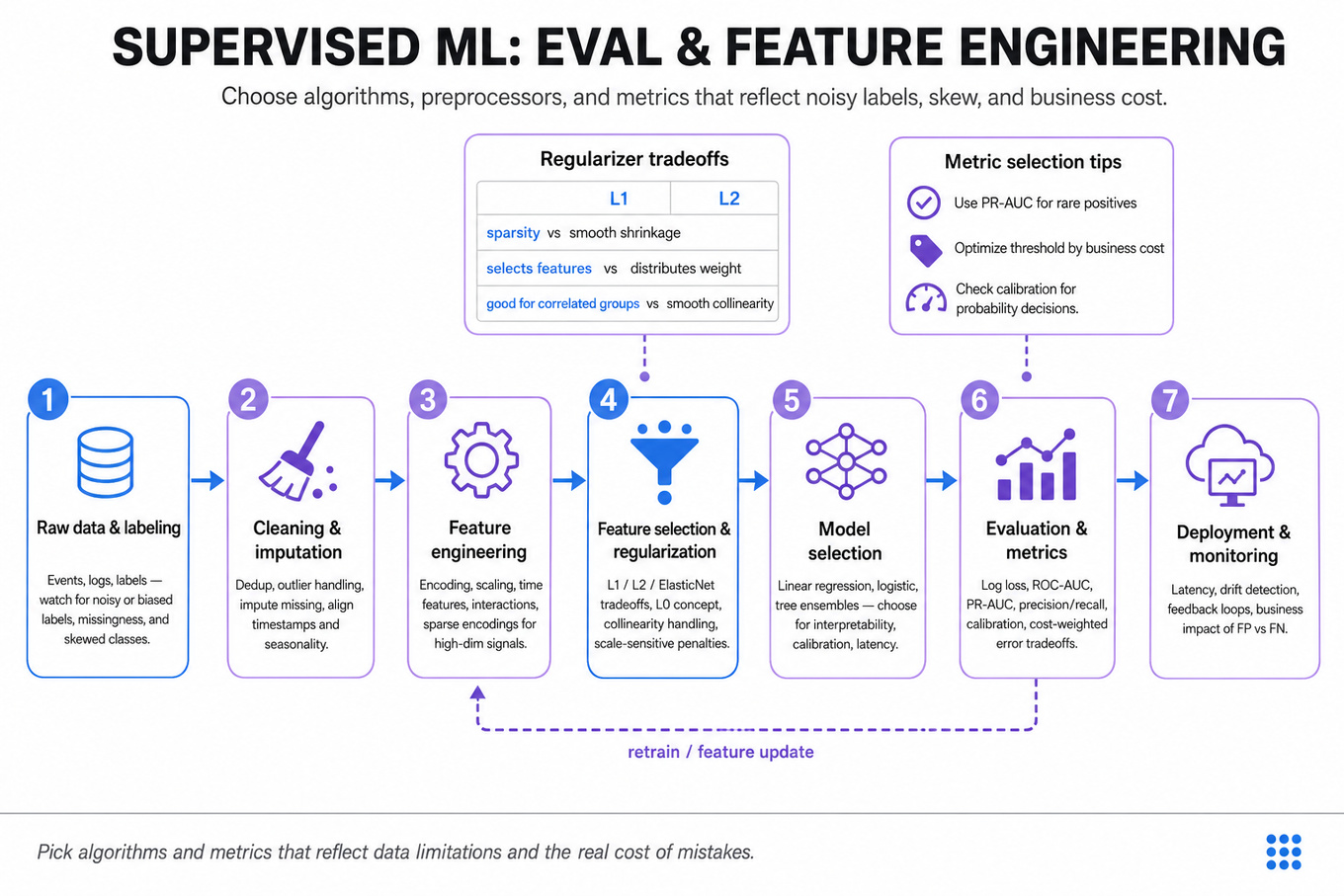
Interviewers are probing whether you can choose, evaluate, and explain supervised learning methods under realistic business constraints: noisy labels, skewed classes, sparse features, correlated predictors, seasonality, and metric tradeoffs. For an Amazon Data Scientist, this matters because many use cases—fraud detection, abuse prevention, conversion modeling, inventory forecasting, search relevance, and customer targeting—require defensible model choices, not just high offline scores. You are expected to reason from the data-generating process, select appropriate algorithms and metrics, identify preprocessing needs, and communicate tradeoffs clearly to product and science partners. The strongest answers connect modeling decisions to customer or business impact, such as false-positive cost, missed-demand cost, latency of decisions, or interpretability needs.

Core knowledge

• Linear regression estimates coefficients by minimizing squared error: $\min_\beta \sum_i (y_i - x_i^\top\beta)^2.$ Its classic assumptions include linearity, independent errors, homoscedasticity, no perfect multicollinearity, and exogeneity $E[\epsilon \mid X]=0$. Violations do not always make predictions useless, but they affect inference, confidence intervals, and coefficient interpretation.

• Logistic regression models class probability as $P(y=1\mid x)=\sigma(x^\top\beta)$ and minimizes log loss, not squared error. It is often a strong baseline for tabular classification, especially when interpretability, calibration, and sparse high-dimensional features matter.

• Regularization controls variance and overfitting by penalizing model complexity. L2 adds $\lambda\|\beta\|_2^2$ and shrinks correlated coefficients smoothly; L1 adds $\lambda\|\beta\|_1$ and can produce sparse feature selection; Elastic Net combines both and is useful with correlated feature groups.

• L0 regularization counts nonzero coefficients, $\|\beta\|_0$, and directly targets feature subset selection, but exact optimization is generally combinatorial. L∞ regularization constrains the maximum absolute coefficient and is less common in applied DS interviews, but tests whether you understand norm geometry and constraint effects.

• Feature scaling is essential for distance-based models, gradient-based linear models, and regularized regression because coefficients are penalized relative to feature scale. Tree models such as Random Forests, Gradient Boosted Trees, `XGBoost`, and `LightGBM` are mostly invariant to monotonic scaling, though transformations can still help with outliers or distribution shape.

• Random Forests reduce variance by bagging many decorrelated trees trained on bootstrap samples and random feature subsets. They are robust, parallelizable, and less sensitive to hyperparameters, but may underperform boosted trees on structured tabular prediction and can struggle with extrapolation beyond observed feature ranges.

• Gradient Boosting sequentially fits trees to residuals or gradients, reducing bias and often winning on tabular data. Key controls are learning rate, number of trees, max depth, subsampling, column sampling, and early stopping. It can overfit label noise if trees are deep or boosting rounds are excessive.

• Class imbalance should be handled through metrics, sampling, thresholds, and cost framing. Accuracy is misleading when positives are rare; prefer precision, recall, F1, PR-AUC, lift, recall at fixed precision, or expected cost. For a 0.1% positive class, ROC-AUC can look strong while precision is unusable.

• Threshold selection is a business decision layered on top of predicted probabilities. A fraud model might optimize expected value: $EV(t)=TP(t)\cdot B - FP(t)\cdot C - FN(t)\cdot L,$ where $t$ is the decision threshold. Always separate model ranking quality from action policy.

• Calibration matters when probabilities feed downstream decisions, capacity planning, or expected-value calculations. Logistic regression is often reasonably calibrated; boosted trees may need Platt scaling or isotonic regression. Evaluate with calibration curves, Brier score, and observed-vs-predicted rates by score bucket.

• Time-series forecasting requires respecting temporal order. Use train/validation splits such as rolling-origin evaluation, not random cross-validation. Baselines should include seasonal naive, moving average, and simple exponential smoothing before complex models like `ARIMA`, `Prophet`, `XGBoost`, or sequence models.

• Feature engineering should encode signal without leakage. For tabular Amazon-style data, common features include lagged demand, rolling means, customer tenure, frequency counts, recency, price bands, categorical target encodings, missingness indicators, and log-transformed monetary values. Compute features using only information available at prediction time.

Tip: In interviews, first state the decision context: “Am I optimizing probability accuracy, ranking quality, forecast accuracy, or a business action threshold?” This prevents generic model comparisons.

Worked example

For Compare Random Forests vs Gradient Boosting rigorously, a strong candidate would start by clarifying the prediction target, data size, feature types, class balance, label noise, interpretability needs, and whether the model is used for ranking, probability estimation, or hard classification. They might say: “I would compare these as two tree-ensemble families: Random Forests primarily reduce variance through bagging, while Gradient Boosted Trees reduce bias through sequential additive learning.” The answer should be organized around four pillars: predictive performance, robustness to noisy or missing data, tuning complexity, and evaluation metrics aligned with the business cost.

For performance, the candidate would explain that boosted trees like `XGBoost` or `LightGBM` often outperform Random Forests on structured tabular data because they iteratively correct errors, but they require careful regularization, learning-rate tuning, and early stopping. For robustness, Random Forests are a safer first pass when labels are noisy or the team needs a stable benchmark with fewer hyperparameters. For feature handling, both can model nonlinearities and interactions, but high-cardinality categoricals may require target encoding, frequency encoding, hashing, or native categorical handling depending on the implementation.

A key tradeoff to flag explicitly is that Gradient Boosting may deliver better PR-AUC or lift in the top score deciles, while Random Forests may be easier to tune and less brittle under distribution shifts. The candidate should also discuss class imbalance: use class weights, balanced sampling, calibrated probabilities, and threshold optimization rather than relying on raw accuracy. A strong close would be: “If I had more time, I’d compare both against a regularized logistic regression baseline, evaluate calibration and segment-level errors, and validate that gains persist on a temporally held-out set.”

A second angle

For Choose Models for Imbalanced Data and Time-Series Forecasting, the same fundamentals apply, but the framing splits into two separate data-generating processes. For the imbalanced classification piece, the central issue is not “which model is most accurate,” but which model ranks rare positives well and supports a defensible action threshold under asymmetric costs. For the forecasting piece, the key constraint is temporal dependence: random splits leak future information and overstate performance. A good answer would compare simple seasonal baselines, `ARIMA`-style models, tree models with lag features, and possibly hierarchical forecasting if predictions aggregate across products, regions, or fulfillment nodes. The transferable skill is matching evaluation design to the operational decision: PR-AUC or recall-at-precision for rare-event detection, and WAPE, sMAPE, pinball loss, or service-level cost for demand forecasts.

Common pitfalls

Pitfall: Treating accuracy as the default classification metric.

This is the most common analytical mistake for imbalanced problems. Saying “the model has 99% accuracy” is weak if the positive class rate is 0.5%; a trivial all-negative classifier gets 99.5% accuracy. A better answer names precision, recall, PR-AUC, top-k lift, calibration, and cost-weighted thresholding.

Pitfall: Reciting model definitions without tying them to data conditions.

A communication mistake is saying “Random Forests are better because they avoid overfitting” or “Gradient Boosting is better because it is more accurate.” Interviewers want conditional reasoning: data size, noise, sparsity, missingness, high-cardinality categoricals, latency constraints, and whether the goal is ranking, calibrated probability, or interpretability.

Pitfall: Ignoring leakage and validation design.

A depth mistake is proposing target encoding, rolling averages, or time-series features without specifying that they must be computed using only past data. For Amazon-style problems with seasonality, promotions, and customer behavior shifts, a random split can make a mediocre model look excellent. Prefer temporal holdouts, grouped splits when entities repeat, and segment-level error checks.

Connections

Interviewers may pivot from here into experiment design, especially how to validate that an offline model improvement translates into an online metric such as conversion, defect rate, or customer contacts. They may also ask about causal inference, ranking metrics like NDCG or MAP, or forecast evaluation under asymmetric costs and stockout penalties.

Further reading

• The Elements of Statistical Learning — rigorous treatment of regularization, tree ensembles, bias-variance tradeoff, and model assessment.

• An Introduction to Statistical Learning — accessible coverage of linear models, classification, resampling, feature selection, and tree-based methods.

• XGBoost: A Scalable Tree Boosting System — foundational paper explaining why regularized gradient-boosted trees became a dominant approach for tabular ML.

Practice questions

Focus area — You marked this exact concept new and selected ranking, recommendation, deployment, rare events, forecasting, and XGBoost topics.

What's being tested

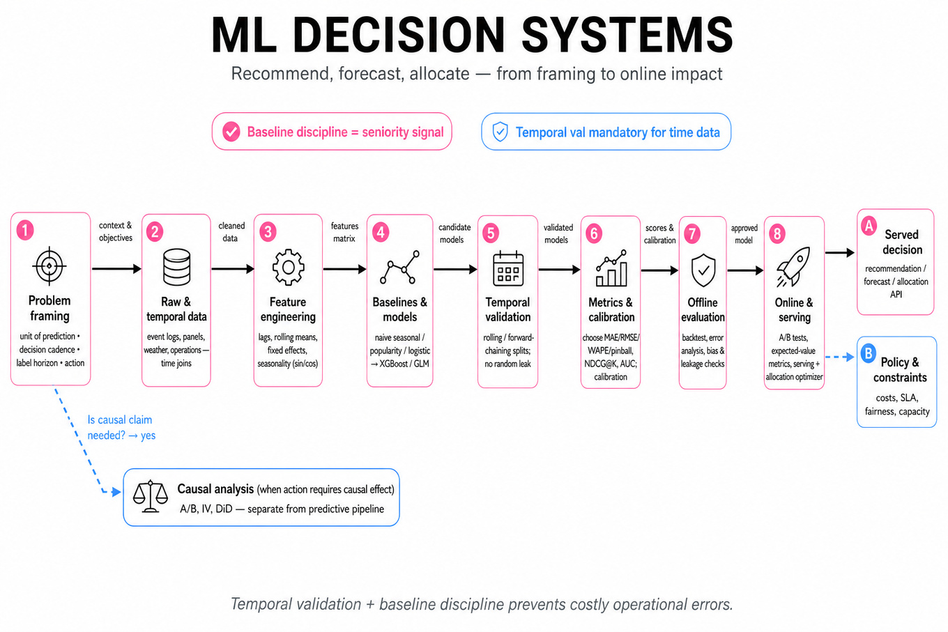
Interviewers are probing whether you can design ML decision systems from a Data Scientist’s lens: define the prediction or causal target, choose defensible features and validation, evaluate offline and online impact, and explain tradeoffs under business constraints. The common thread is not “build a model,” but “turn messy behavioral, temporal, or operational data into a reliable decision: recommend this item, forecast this demand, allocate this courier, estimate this treatment effect.” Amazon cares because small errors in ranking, forecasting, churn prediction, and fulfillment allocation compound across millions of customers, packages, and marketplace interactions. A strong answer shows statistical discipline: avoiding leakage, validating temporally, separating prediction from causal claims, and choosing metrics aligned with customer experience and cost.

Core knowledge

• Problem framing comes first: define the unit of prediction, decision cadence, label horizon, and action. For churn, that may be “probability a subscriber cancels in the next 30 days”; for allocation, “expected service time if courier $c$ receives package $p$ at time $t$.”

• Temporal validation is mandatory for forecasting, churn, recommendations, and logistics. Use rolling or forward-chaining splits rather than random splits: train on weeks 1–8, validate on week 9, test on week 10. Random splits leak seasonality, user lifecycle, and future availability.

• Forecasting panel data combines cross-sectional and time-series signals. For utility consumption, model household/account fixed effects, weather, holidays, lagged usage, rolling means, and seasonality terms such as $\sin(2\pi t/365)$ and $\cos(2\pi t/365)$. Compare against naive seasonal baselines before complex models.

• Baseline discipline is a major signal of seniority. For energy demand, include last-week-same-hour or same-month-last-year baselines; for recommendations, popularity and recently viewed items; for churn, logistic regression. If XGBoost beats a weak baseline only, the result is not convincing.

• Metric choice should match the decision. Regression may use MAE, RMSE, WAPE, or pinball loss; ranking may use NDCG@K, MAP@K, recall@K, and diversity; churn uses AUC, precision-recall, calibration, and lift. Cost-sensitive settings require expected value, not just accuracy.

• Calibration matters when predictions drive thresholds or optimization. A churn model with good AUC can still overstate risk; use reliability plots, Brier score, or isotonic/Platt calibration. Allocation systems need predicted durations and uncertainty, not only rank order.

• Feature leakage is the most common hidden failure. Examples: using “delivery completed timestamp” to predict package allocation, post-cancellation support contacts to predict churn, or future weather actuals in an energy forecast. Every feature should be available at decision time.

• Missing data is a signal and a risk. Distinguish MCAR, MAR, and MNAR; add missingness indicators when absence is behaviorally meaningful, impute within training folds, and avoid target-aware imputation. For subscription churn, missing billing or engagement fields may indicate disengagement.

• Double Machine Learning estimates causal effects with flexible nuisance models while reducing regularization bias. For outcome $Y$, treatment $D$, covariates $X$, residualize: $\tilde{Y}=Y-\hat{m}(X)$ and $\tilde{D}=D-\hat{e}(X)$, then estimate $\hat{\theta}=\frac{\sum_i \tilde{D}_i\tilde{Y}_i}{\sum_i \tilde{D}_i^2}.$ Use cross-fitting to avoid overfitting nuisance functions.

• Text and address-derived features can be useful but risky. TF-IDF, geohashes, learned embeddings, or parsed address components may proxy for socioeconomic status or geography. Validate representation quality, check overlap/positivity, test sensitivity to feature removal, and discuss fairness or compliance concerns.

• Recommender systems are usually staged: candidate generation, ranking, filtering, and evaluation. A DS should focus on relevance labels, negative sampling, counterfactual bias, offline metrics, segment performance, and experiment design—not low-level serving mechanics. Watch for position bias and popularity bias.

• Allocation models often combine prediction with optimization. Predict service time, failure probability, or lateness risk, then optimize an objective such as $\min \sum_{p,c} x_{pc}\hat{t}_{pc}$ subject to courier capacity, route feasibility, promised delivery windows, and fairness constraints. Evaluate both model error and operational outcomes.

Worked example

For Build a package-allocation model for couriers, start by clarifying the decision: “Are we assigning packages to couriers once per shift, continuously during the day, or at dispatch waves? Is the goal to minimize late deliveries, total route time, cost, or customer promise misses?” Then declare assumptions: each package has location, size, promised delivery window, and historical stop features; each courier has capacity, current route context, region familiarity, and shift constraints.

A strong answer can be organized into four pillars: prediction target, feature design, optimization layer, and evaluation. First, model per-stop service time or lateness probability using historical package-courier-route observations, with features like building type, delivery density, time of day, package size, weather, and courier experience in that area. Second, validate temporally and geographically, because performance on familiar neighborhoods may not generalize to new routes or seasonal peaks.

Third, feed predictions into a constrained assignment objective: minimize expected lateness or total cost while respecting capacity, route duration, promised windows, and workload balance. Fourth, evaluate offline with MAE for service time, calibration for lateness probabilities, and simulated operational metrics such as late-package rate, packages per courier hour, and customer-contact rate. The explicit tradeoff to flag is interpretability versus accuracy: a gradient-boosted model may forecast service time well, but simpler additive effects may be easier to debug when couriers or stations report implausible assignments. Close by saying: “If I had more time, I would add uncertainty-aware allocation, stress-test peak-season cohorts, and run an A/B test against the current dispatch heuristic with guardrails on late deliveries and courier workload.”

A second angle

For Apply Double ML with text-address features, the same discipline applies, but the target is causal rather than predictive. Instead of asking “Can text/address features predict the outcome?”, ask whether they adequately control confounding without violating overlap or encoding problematic proxies. The answer should frame treatment, outcome, covariates, and estimand—usually ATE or CATE—then explain cross-fitting, nuisance models for treatment and outcome, and residual-on-residual estimation. The key difference is evaluation: high predictive accuracy is insufficient; you need balance diagnostics, overlap checks, placebo tests, sensitivity analysis, and confidence intervals. Text embeddings may improve confounding control, but they can also make causal assumptions less transparent.

Common pitfalls

Pitfall: Treating every problem as a pure supervised-learning leaderboard.

A tempting answer is “I’d train XGBoost, tune hyperparameters, and optimize AUC or RMSE.” That misses the business decision. Allocation requires constraints and operational simulation; recommendations require ranking and online behavior; causal questions require identification assumptions, not just prediction.

Pitfall: Communicating a system design answer like an ML engineer.

For a Data Scientist, do not spend most of the answer on Kafka, feature-store plumbing, request fanout, or deployment topology. It is fine to mention that features must be available at decision time, but the stronger discussion is about labels, leakage, validation windows, objective functions, bias, calibration, and experiment design.

Pitfall: Ignoring segment-level and temporal failure modes.

Aggregate metrics can hide failures for new users, rural addresses, peak-season weeks, cold-start items, or high-value customers. A better answer says upfront that you would report metrics by cohort, geography, tenure, traffic source, item category, weather regime, or delivery station, depending on the product.

Connections

Interviewers may pivot from here into experimentation, especially A/B testing recommender or allocation changes with guardrail metrics like cancellation rate, late delivery rate, or customer contacts. They may also probe causal inference, time-series forecasting, ranking evaluation, fairness, or model monitoring from a metric and decision-quality perspective.

Further reading

• “Double/Debiased Machine Learning for Treatment and Structural Parameters” — Chernozhukov et al., 2018 — foundational paper for residualization, orthogonalization, and cross-fitting in causal ML.

• “Recommender Systems Handbook” — Ricci, Rokach, and Shapira — broad coverage of ranking, evaluation, cold start, and recommender tradeoffs.

• “Forecasting: Principles and Practice” — Hyndman and Athanasopoulos — practical reference for baselines, cross-validation, seasonality, and forecast accuracy metrics.

Practice questions

Coding & Algorithms

Focus area — Coding is 1/5 and you marked many patterns new: DP, graphs, heaps, sliding windows, hash maps, two-pointers, and string DP.

What's being tested

Amazon MLE coding screens test whether you can turn ML-adjacent production tasks into clean algorithms: batching, clustering, training loops, graph reachability, interval allocation, and top-k retrieval. Interviewers look for correct data structures, complexity analysis, edge-case handling, and code that would survive inside a training or serving pipeline.

Patterns & templates

• K-means implementation — initialize centroids, assign by nearest distance, recompute means; stop on max iterations or centroid shift $\lt \epsilon$.

• Interval merging / allocation — sort by start time, scan once, merge or consume ranges; usually O(n log n) time from sorting.

• Top-k frequency retrieval — use collections.Counter plus heapq.nlargest for O(n log k), or bucket counts for bounded frequencies.

• Directed cycle check — adding edge u -> v creates a cycle iff u is reachable from v; solve with DFS/BFS.

• PyTorch training loop — order matters: model.train(), move tensors to device, optimizer.zero_grad(), forward, loss, backward(), step().

• Bucket batching optimization — sort or group examples by sequence length/cost, then pack batches to reduce padding and GPU underutilization.

• Event-driven queues — model backorders or pending work with deque, heapq, or ordered maps; define FIFO vs priority semantics explicitly.

Common pitfalls

Pitfall: Writing ML pseudocode without executable edge handling, such as empty clusters in K-means or zero-length batches in bucketing.

Pitfall: Missing complexity tradeoffs; Amazon interviewers expect O(V+E), O(n log n), memory cost, and when the approach breaks at scale.

Pitfall: In PyTorch loops, forgetting optimizer.zero_grad() or device movement silently produces wrong training behavior or runtime errors.

Practice these

The practice cards below cover the canonical variants — solve all of them and time yourself.

Practice questions