Waymo Data Scientist Interview Prep Guide

Focus most on Waymo-shaped statistics, experimentation, SQL ride analytics, and robust coding because every category is self-rated 3/5 and there are no solved-question signals yet. Your skipped concept ratings default to solid, so narrower standalone topics like K-means, finite-population sampling, and Monte Carlo probability are kept brief rather than treated as gaps. The Waymo-specific emphasis is on autonomous-vehicle safety metrics, trajectory and collision analysis, geospatial/spatiotemporal confounding, simulation scenario mining, sensor-label quality, and safety-first leadership. With one month, use this as a two-pass plan: first cover every emphasized concept, then rotate through normal concepts with timed SQL, experimentation, and stats drills.

Take-home Project — 33 min

Data Manipulation (SQL/Python)

Analytics & Experimentation

Focus area — Existing outline covers the Waymo safety addendum; bumped up for rare, high-severity autonomous-vehicle outcomes.

What's being tested

Interviewers probe your ability to operationalize safety: define measurable, statistically sound metrics for rare adverse events, design experiments/analyses that can detect meaningful changes, and reason about uncertainty and tradeoffs when data are sparse. For Waymo, this maps to showing you can turn telemetry and human-intervention logs into defensible statements about change in risk, choose appropriate statistical models for low-count events, and communicate uncertainty to engineering and product partners.

Core knowledge

• Unit of analysis (exposure) — choose between trip, mile, hour, or scenario-exposure; denominators drive interpretability and power. Always state the exposure used and why (e.g., miles normalizes for routing).

• Primary safety metrics — common choices: collision_rate (events per million miles), intervention_rate (operator or fallback interventions per 100k miles), and near-miss proxies (time-to-collision distributions, hard-brake events). Define event, dedup rules, and attribution windows.

• Rare-event modelling — treat discrete counts with Poisson (mean≈variance) or negative binomial for overdispersion; use zero-inflated models if many zeros. For count k over exposure T: rate r = k/T and Var(r)≈k/T².

• Exact inference for small counts — use exact Poisson or exact binomial CI (chi-square inversion) rather than normal approximations when k is small (k<10). For testing, use exact rate ratio tests or conditional Poisson tests.

• Power and sample-size for rates — approximate exposure T required to detect an absolute rate difference Δ: $T \approx \frac{(z_{1-\alpha/2}+z_{1-\beta})^2(\lambda_1+\lambda_2)}{\Delta^2}$ where λ are rates per unit exposure. For tiny baseline rates, required T often scales to millions/billions of miles.

• Sequential / online testing — use alpha-spending or group-sequential methods (e.g., O’Brien–Fleming) for repeated looks; for safety-critical launches prefer pre-specified stopping rules and conservative corrections.

• Confounding & causal inference — control for exposure mix (urban vs. highway), weather, time-of-day, and driver takeover propensity via stratification, matching, or weighted regression; randomized A/B is ideal for software stacks but often impractical.

• Composite & leading indicators — combine rare crash metrics with higher-rate proxies (e.g., hard_brake_rate) using composite scores or hierarchical models to increase sensitivity while preserving interpretability.

• Hierarchical / Bayesian models — borrow strength across segments (vehicle version, route type) with random effects to stabilize low-count estimates and get better posterior intervals for rates.

• Multiple comparisons & FDR — when evaluating many routes/scenarios, correct using Benjamini–Hochberg for false-discovery control or adjust family-wise error for conservative safety statements.

• Evaluation windows & latency — decide on event attribution lookback windows, handle late-arriving reconciliations as measurement error, and quantify how delayed labeling affects power and bias.

Tip: Always report both absolute and relative changes (e.g., drop of 0.0002 events/mile = 20% relative) and include exposure units so stakeholders can reason about operational impact.

Worked example — "Design a safety metric for AV interventions"

Frame: In the first 30 seconds ask: what counts as an intervention (human take-over vs autopilot fallback), what is the exposure unit (miles vs trips), and which populations/ODDs (operational design domains) to include. Skeleton answer pillars: (1) precise event definition and dedup rules, (2) denominator choice and stratification plan, (3) statistical model and expected baseline rate, (4) power/sample-size and rollout testing plan, (5) monitoring and alerting thresholds. Tradeoff: choosing miles normalizes exposure but can hide scenario-specific risk (e.g., intersections per mile); call out a plan to report both intervention_rate_per_mile and intervention_rate_per-intersection. Close by stating validation steps (manual label audits, synthetic injection tests) and what you'd do with more time: estimate required miles to detect a 20% reduction using historical intervention_rate and fit a hierarchical Poisson model to borrow strength across cities.

A second angle — "Estimate miles required to detect a 10% reduction in collision rate"

Here the same primitives apply but constraints change: this is a power calculation for very rare events. Start by estimating baseline rate λ (e.g., collisions per million miles) and variance model (Poisson vs overdispersed). Use the exposure formula (see Core knowledge) to solve for required T; communicate results as orders of magnitude (e.g., “you need O(10⁸–10⁹) miles for small relative reductions”), and present alternatives: use composite endpoints including near-misses, extend study by synthetic scenario testing in simulation, or run paired comparisons within controlled ODDs to increase signal. Emphasize cost–benefit: if required miles are infeasible, propose higher-signal proxies or staged evaluation.

Common pitfalls

Pitfall: Misdefining denominator — reporting change in absolute count without normalizing for exposure (fewer miles driven leads to fewer events but not safer behavior). Always pair counts with exposure and normalized rates.

Pitfall: Normal-approximation mistakes — using z-tests/CIs for Poisson counts when k is very small leads to anti-conservative p-values. Use exact or Poisson-based intervals for small k.

Pitfall: Overclaiming causality — presenting uncontrolled before/after comparisons as evidence of safety improvement; state confounders, show stratified analyses, or use randomized/controlled designs when possible.

Connections

This topic naturally pivots to simulation validation (how simulation-derived risk correlates with field metrics), anomaly detection for incident triage, and causal inference (instrumental variables, difference-in-differences) when randomized experiments aren’t possible.

Further reading

• [Regression Analysis of Count Data — Cameron & Trivedi] — authoritative coverage of Poisson, negative binomial, and overdispersion modeling useful for rare-event counts.

• [An Introduction to the Bootstrap — Efron & Tibshirani] — practical bootstrap techniques for constructing confidence intervals when analytic approximations fail.

Practice questions

Statistics & Math

Recurring across all rounds; statistics is 3/5 with views but no solved signals, so keep inference warm.

What's being tested

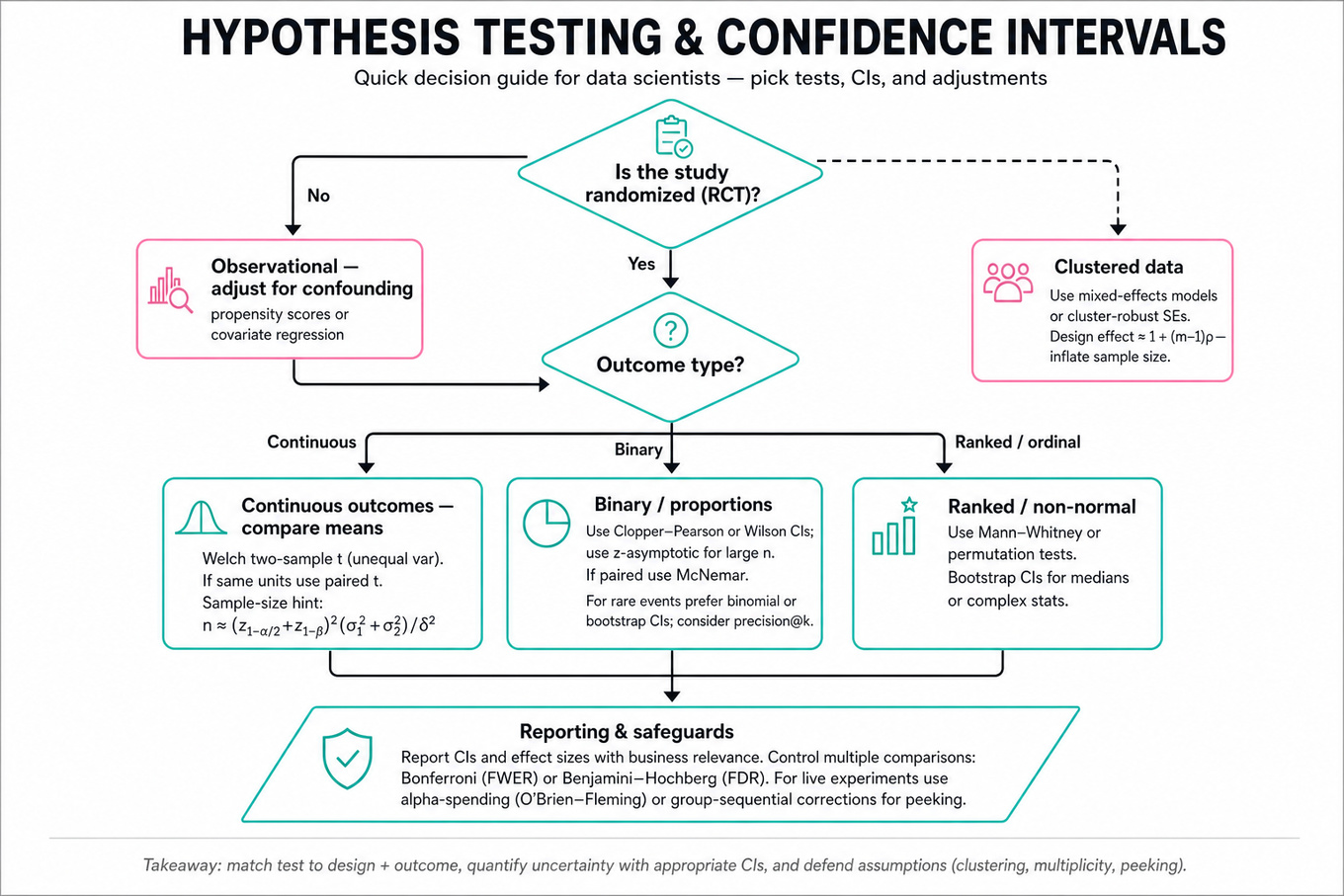
Interviewers are probing your ability to turn noisy observational or experimental data into defensible statements about causal effects and uncertainty: choosing an appropriate test, estimating confidence intervals, and diagnosing threats to validity. For Waymo this matters for routing, safety, and model-rollouts where small real-world differences matter and rare events or repeated measures complicate inference. Expect to justify metric choices, sampling/exclusion rules, and statistical assumptions quickly.

Core knowledge

• Randomized controlled trial (RCT) vs. observational analysis: RCTs support causal claims under randomization; observational requires explicit confounding adjustment (propensity scores, covariate regression).

• Intent-to-treat (ITT) vs per-protocol: ITT preserves randomization for unbiased effect on assignment; per-protocol estimates treatment-on-treated but can be biased by post-randomization selection.

• Welch t-test and two-sample t: use for comparing means with unequal variances; sample-size formula: $n\approx\frac{(z_{1-\alpha/2}+z_{1-\beta})^2(\sigma_1^2+\sigma_2^2)}{\delta^2}$ where $\delta$ is detectable difference.

• Nonparametric tests: use Mann–Whitney for distributional shifts, permutation tests for exact randomization inference, and bootstrap CIs for medians or complex statistics.

• Confidence intervals (CI) for proportions: use Clopper–Pearson or Wilson for small counts; for differences use asymptotic z or bootstrap when assumptions fail.

• Rare-event metrics: prefer precision@k, FDR-controlled lists, and report CIs using binomial or bootstrap; beware unstable AUC with tiny positives.

• Paired comparisons: when the same units appear in both conditions use paired t or McNemar's test for binary outcomes to leverage reduced variance.

• Clustered data: account for cluster correlation via mixed-effects models or adjust variance with cluster-robust SEs; design effect ≈ $1+(m-1)\rho$ inflates required sample size.

• Multiple comparisons: control FWER with Bonferroni or FDR with Benjamini–Hochberg when testing many metrics or segments.

• Sequential testing: live experiments require alpha-spending or sequential correction (e.g., O’Brien–Fleming, group-sequential) to avoid inflated Type I error if you peek.

• Effect size & business relevance: report absolute and relative effects plus standardized Cohen’s d; combine CI width and minimum detectable effect to argue practical significance.

• Assumption checks: visualize distributions, check balance by key covariates, test homoskedasticity, and inspect time trends for pre-existing drift or spillovers (violations of SUTVA).

Worked example — Test Whether a Routing Experiment Reduced Pickup Time

First 30s: ask whether randomization unit is trip, driver, or region; how pickup time is defined (request-to-arrival?), treatment assignment timing, and whether there are repeated rides per user or driver. Skeleton answer pillars: (1) Define primary metric and exclusions (e.g., canceled rides, extreme outliers), (2) Data join & deduplication to ensure independent units (or identify clusters), (3) Choose test and CI (Welch t on mean pickup-time or log-transform + bootstrap median CI), (4) Sensitivity checks (ITT, per-protocol, covariate-adjusted regression, cluster-robust SE). A key tradeoff: mean pickup time is sensitive to skew and rare long waits — median gives robust central tendency but smaller policy-relevant differences; choose based on stakeholder loss function. Close by proposing diagnostics: check balance, pre-period trends, subgroup effects, and if more time—run permutation test, mixed-effects model with driver random intercept, and a pre-specified sequential plan.

A second angle — Compare two rare-event detection models statistically

Here the core concept (inference under small counts) is the same but constraints differ: labels are highly imbalanced and evaluation focuses on precision/recall at operating points, not overall means. Use paired evaluations on the same test set and report CIs for sensitivity using Clopper–Pearson, and for differences use bootstrap paired resampling or McNemar on thresholded outputs. If positive labels are extremely scarce, avoid AUC variance approximations; instead do exact/binomial tests and show precision@k with bootstrap CIs. Also consider cost-weighted metrics and decision-theoretic thresholds when reporting statistically significant but operationally negligible improvements.

Common pitfalls

Pitfall: Treating non-normal, skewed time metrics with a t-test without transformation or robust alternatives. This yields misleading p-values and CIs — use log transforms, median+bootstrap, or permutation tests and show both mean and median results.

Pitfall: Ignoring clustering or repeated measures (e.g., multiple rides per user). Naively treating observations as i.i.d. underestimates SEs; adjust with cluster-robust SEs, mixed models, or aggregate-per-unit.

Pitfall: Overemphasizing p-values and not stating practical significance. A tiny but highly significant mean reduction may be irrelevant operationally; always report CIs, absolute effect, baseline rate, and estimated ROI or safety impact.

Connections

Interviewers may pivot to causal inference (instrumental variables, difference-in-differences), sequential/online experimentation (alpha-spending, bandits), or survival/time-to-event analysis (Kaplan–Meier, Cox models) for metrics like time-to-pickup and rare safety incidents.

Further reading

• [Practical Guide to Controlled Experiments on the Web — Kohavi et al., Microsoft (2009)](Kohavi et al. 2009) — pragmatic lessons on experiment design, metrics, and pitfalls.

• [Bootstrap Methods and Their Application — Davison & Hinkley](Davison & Hinkley) — solid reference for bootstrap CIs and resampling strategies.

Practice questions

Coding & Algorithms

Take-homes and screens reward clean edge-case handling; coding is 3/5 with no solved signals, so practice deliberately.

What's being tested

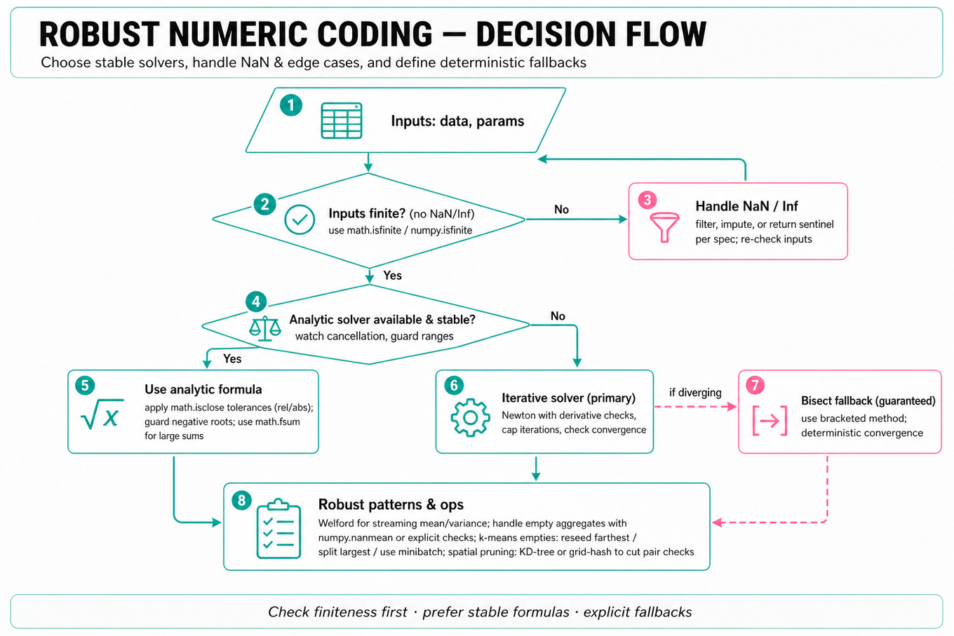
These problems test numeric stability and robust handling of edge cases in algorithmic code: correct use of analytic vs iterative solvers, safe aggregation over missing/empty data, and cluster-maintenance strategies. Interviewers expect concise, production-ready code that handles NaNs, extreme values, degenerate geometry, and streaming inputs.

Patterns & templates

• Pairwise quadratic solver for moving-object collisions — solve $distance^2(t)=r^2$ as $at^2+bt+c=0$, handle discriminant $\le0$, use math.isclose tolerances.

• Use analytic formulas where stable; prefer math.fsum over sum for large numerics to avoid loss of precision.

• Welford's algorithm for streaming mean/variance — single pass, O(1) memory, numerically stable incremental updates.

• For empty/missing values, prefer numpy.nanmean or explicit checks with math.isnan/math.isfinite and return 0 or sentinel per spec.

• Root-finding fallbacks: use bisect (guaranteed convergence) when Newton's method diverges; always cap iterations and check derivative magnitude.

• K-means empty-cluster handling: re-seed with farthest point, split largest cluster, or use minibatch to avoid empties; document deterministic tie-breaks.

• Spatial pruning: use grid hashing / KD-tree / sweep-line to reduce $O(n^2)$ pair checks to near-linear in sparse scenarios.

• Use relative vs absolute tolerance: compare with $abs(a-b) \le max(rel\_tol \cdot max(|a|,|b|), abs\_tol)$ (implement via math.isclose).

Common pitfalls

Pitfall: Treating NaN or infinite values as numbers — forgetting math.isfinite leads to silent wrong answers or crashes.

Pitfall: Using naive sum for long lists — leads to catastrophic cancellation; prefer math.fsum or compensated summation.

Pitfall: Returning any root from quadratic without checking time bounds or negative times — report earliest non-negative collision only.

Practice these

The practice cards below cover the canonical variants — solve all of them and time yourself.

Practice questions

Technical Screen — 36 min

Statistics & Math

Focus area — Highly Waymo-specific motion reasoning; 3/5 stats/coding and no solved signals justify extra practice.

What's being tested

Interviewers probe your ability to convert vehicle motion into analyzable mathematical objects, select appropriate statistical or numerical methods, and reason about uncertainty and scale. They expect clear problem framing (assumptions, observables), correct kinematic modeling (relative motion → algebraic root problems or time-series comparisons), and principled evaluation metrics that capture safety-relevant errors. For Waymo, the focus is on defensible, reproducible analysis (false positive/negative tradeoffs, calibration) rather than low-level sensor plumbing.

Core knowledge

• Relative motion reduction: For two objects with positions p1(t), p2(t), define relative position r(t)=p1(t)-p2(t); collision when $|r(t)| ≤ R$ (sum of radii). Squared-distance $d^2(t)=r(t)·r(t)$ is the central scalar function to analyze.

• Quadratic closed-form case: If each object moves linearly (p(t)=p0+v t), then $d^2(t)=a t^2 + b t + c$; solve $a t^2 + b t + (c-R^2) ≤ 0$ via discriminant $\Delta=b^2-4a(c-R^2)$. Real roots → collision interval; $\Delta≈0$ → grazing/tangent contact.

• Numerical root-finding: For higher-order/parametric trajectories (splines, polynomials), use robust solvers (brentq, Brent’s method) on $d^2(t)-R^2$ with bracketed intervals; prefer bracketed methods over pure Newton to avoid divergence.

• Piecewise models & monotonicity: Break trajectories into segments where motion model is simple (constant velocity/acceleration or low-order spline). Solve per-segment and merge intervals — avoids global multimodality pitfalls.

• Discrete sampling & interpolation: Real logs are sampled; use sinc-compatibility thinking: ensure interpolation (linear / cubic spline) doesn't introduce spurious crossings. Report resolution-limited uncertainty: sample interval $\Delta t$ sets minimum resolvable time-to-collision.

• Uncertainty propagation: For Gaussian position noise, linearize root solution to approximate time uncertainty via the implicit function theorem, or compute confidence intervals via bootstrap or Monte Carlo perturbation of trajectories.

• Scalability & candidate filtering: Naive pairwise is $O(N^2)$; for $N$ up to a few hundred (typical road scene) it's fine, but for thousands use spatial bucketing / R-tree-style prefiltering or coarse time-to-contact heuristics to prune pairs. Document assumptions about upstream sampling frequency.

• Trajectory comparison metrics: For comparing turns use Dynamic Time Warping (DTW), Fréchet distance, or functional summaries (curvature, yaw-rate, lateral displacement) and model differences with mixed-effects or permutation tests to control vehicle-level correlation.

• Statistical testing & multiple comparisons: When testing many segments/cohorts, correct p-values using Benjamini–Hochberg or conservative Bonferroni depending on FDR vs family-wise error tradeoffs.

• Evaluation metrics for collision prediction: Use precision–recall curves and area under PR (AUPR) for imbalanced events; report time-error metrics like MAE of predicted time-to-collision and calibration curves for estimated probabilities.

• Edge cases: Handle initial overlaps (collision at $t=0$), tangential grazes ($\Delta≈0$ numerical sensitivity), and very-high-speed/low-radius pairs that amplify discretization and floating-point errors.

• Safety-aware thresholds: For alarm systems, preferring higher recall (catch all imminent collisions) may be mandated; quantify business cost with a simple cost matrix and optimize thresholds accordingly.

Tip: Always state whether you assume continuous-time analytic trajectories or discrete logged samples — it determines analytic vs numerical solution choices.

Worked example — Determine earliest collision among moving cars

First 30s framing: ask what observables you have (position, velocity, vehicle radii, sample rate), what motion model is acceptable (constant velocity, constant accel, or spline-interpolated), and the time window of interest. Skeleton answer pillars: (1) reduce to per-pair relative-position problem r(t) and $d^2(t)$, (2) choose solver: closed-form quadratic if linear motion, otherwise bracketed numerical root-finding per segment, (3) scale/prune candidate pairs and quantify uncertainty. A strong candidate explicitly handles initial overlap and tangency: check $c-R^2 ≤ 0$ at $t=0$ (immediate collision), and treat $\Delta≈0$ with a tolerance epsilon tied to measurement noise. Tradeoff to flag: using high-order spline interpolation reduces discretization error but can create oscillatory artifacts and expensive root-finding; prefer piecewise low-order fits with adaptive sampling. To close: report earliest collision time with confidence interval, show complexity ($O(M)$ segments × pairs after pruning), and say "if I had more time, I'd add Monte Carlo uncertainty quantification and a labeled holdout to estimate false positive rate under realistic sensor noise."

A second angle — How compare Waymo turning trajectories statistically

Here the task shifts from pairwise collision roots to population-level comparison of turning behavior. Apply the same fundamental reduction: represent each trajectory as a time-indexed function (x(t), y(t)) or as a path in Frenet frame (longitudinal vs lateral offset relative to lane center). Extract interpretable features: curvature $\kappa(t)$, yaw-rate, lateral displacement at matched arc-length, and time-normalized speed profiles. Use functional-data techniques (mixed-effects models or Gaussian Process regression) to model per-vehicle random effects and test treatment/cohort fixed effects (autonomous vs baseline). For non-time-aligned turns, use DTW or elastic registration to align phases before averaging; when you report significance, correct for vehicle-level clustering (cluster-robust SEs) and multiple segments. The common concept — converting raw trajectories to analyzable functions and choosing alignment + appropriate null distribution — carries across both tasks.

Common pitfalls

Pitfall: Assuming closed-form quadratics everywhere. Many real-world trajectories are non-linear or spline-interpolated; blindly applying the quadratic formula will miss collisions or produce imaginary roots.

Pitfall: Ignoring sampling resolution and noise when reporting collision time. Claiming sub-millisecond precision without uncertainty quantification or sensor-rate justification undermines credibility.

Pitfall: Using pointwise t-tests on time-series without accounting for temporal correlation or vehicle-level clustering; this inflates false positives. Use functional tests, mixed models, or permutation strategies.

Connections

These analyses commonly pivot to trajectory clustering and anomaly detection, time-to-collision (TTC) modeling and calibration, and probabilistic filtering like the Kalman filter for state estimation. Interviewers may also ask to validate models with holdout scenarios or to design experiments that measure behavioral change after a software update.

Further reading

• [Brent, R.P., "Algorithms for Minimization Without Derivatives"] — reliable reference for robust 1-D root-finding (bracketing methods).

• [Ramsay & Silverman, "Functional Data Analysis"] — practical methods for representing and testing differences between trajectories.

Practice questions

• Hypothesis Testing And Confidence Intervals — covered in depth under Take-home Project below.

Machine Learning

• Sensor Data Quality And Label Analytics (Focus) — covered in depth under Onsite below.

Coding & Algorithms

• Robust Coding And Numeric Edge Cases — covered in depth under Take-home Project below.

Data Manipulation (SQL/Python)

Analytics & Experimentation

• Autonomous Vehicle Safety Metrics (Focus) — covered in depth under Take-home Project below.

Onsite — 30 min

Analytics & Experimentation

• Autonomous Vehicle Safety Metrics (Focus) — covered in depth under Take-home Project below.

Machine Learning

Focus area — New Waymo-specific addendum for perception data quality, annotation reliability, and drift not covered by base ML topics.

What's being tested

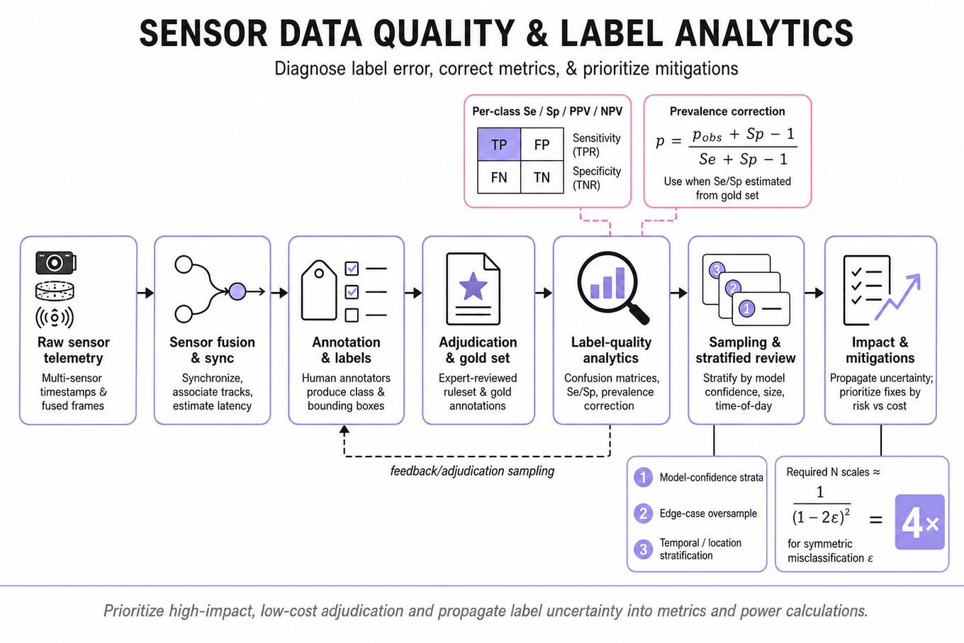
Interviewers are probing your ability to treat sensor telemetry and annotated labels as noisy measurement systems: quantify how measurement error affects key metrics, design sampling/adjudication to diagnose root cause, and recommend actionable mitigations that trade cost for statistical confidence. For Waymo, this matters because model decisions and safety metrics are computed from multi-sensor fused signals and human labels; the candidate must show rigorous statistical reasoning, experiment design, and metric-driven prioritization — not systems plumbing or labeler management.

Core knowledge

• Label noise: random vs systematic noise; random adds variance and attenuates effect sizes, systematic creates bias. Model evaluation must separate the two to avoid misleading conclusions.

• Confusion matrix: use per-class sensitivity (TPR), specificity (TNR), precision (PPV), and negative predictive value (NPV) to reason about observed vs true rates; label error changes both numerator and denominator.

• Prevalence correction: if annotator sensitivity Se and specificity Sp are estimated, true prevalence p relates to observed prevalence p_obs as
  $p=\frac{p_{obs} + Sp -1}{Se + Sp -1}$
  Use when gold adjudication yields Se/Sp for noisy labels.

• Annotator models: Dawid–Skene / EM estimates per-annotator confusion matrices and latent true labels; works for thousands of items but may overfit with few repeats — regularize or group annotators.

• Agreement metrics: Cohen's kappa (pairwise), Krippendorff's alpha (multi-annotator, missing labels); interpret values contextually (0.6 may be fine for hard perception tasks).

• Sampling & stratification: design stratified review by model confidence, edge-case flags, object size, time-of-day; prioritized sampling uncovers rare but important failure modes efficiently.

• Adjudication design: use a gold set (expert-reviewed) vs majority-vote; for safety-critical labels prefer expert adjudication with documented rules, and measure inter-adjudicator agreement.

• Impact on experiments: misclassification attenuates treatment effects in A/B tests; required sample size increases by factor roughly $1/(1 - 2\epsilon)^2$ for symmetric misclassification rate $\epsilon$. Always propagate label uncertainty into power calculations.

• Covariate vs label shift: distinguish covariate shift (p(x) changes) from label shift (p(y) changes) and conditional shift (p(y|x) changes); detection methods differ (density-ratio estimation vs confusion-matrix calibration).

• Metric instrumentation: compute per-segment metrics (by sensor, lighting, object distance) and time-windowed metrics (p95, p99) to localize degradation; global aggregates often hide critical slices.

• Noise-aware model evaluation: consider training with noise-robust losses, label smoothing, or reweighting by annotator reliability; evaluate on a reserved adjudicated test set, not noisy training labels.

• Cost-effectiveness: quantify marginal value of more adjudication by modeling uncertainty reduction per adjudicated label and compare to expected safety or metric improvement.

Worked example — "Quantify labeler agreement and its impact on model performance"

First 30s: ask whether labels are multi-class or binary, whether multiple annotators per item exist, what adjudication standard (expert) is available, and the prevalence of positive cases. Skeleton: (1) estimate per-annotator confusion matrices from a doubly-labeled subset; (2) use Dawid–Skene or simple majority to infer latent truth and compute Se/Sp; (3) propagate Se/Sp into corrected precision/recall using the prevalence correction and adjusted confusion formulas; (4) design targeted adjudication on slices where annotator disagreement or model uncertainty is high. Key tradeoff: full adjudication gives unbiased metrics but is expensive — prioritize items that most affect safety metrics (e.g., low-confidence pedestrian detections at night). Close by noting you'd run a power analysis to decide adjudication budget and, if time allows, simulate the effect of different adjudication rates on downstream metric variance.

A second angle — "Detect and diagnose sensor-quality regressions that change validation metrics"

Here the framing shifts from labeler error to upstream sensor degradation manifesting as changed label distributions. Approach: (1) compare per-sensor and per-hardware-version slices over time, adjusting for traffic/context; (2) use unlabeled-signal drift detectors (e.g., feature-distribution divergence like KL or MMD) and correlate detected drift with rises in annotation disagreement or drops in per-slice precision; (3) run a targeted labeling push on periods flagged by drift detectors to confirm if label distribution or annotator confusion changed. The same statistical tools (confusion matrices, stratified sampling, adjudication) apply, but constraints emphasize temporal causality and faster triage.

Common pitfalls

Pitfall: Treating labels as ground truth.
Analytical mistake: reporting model precision/recall on noisy labels without quantifying annotator error leads to overconfidence or false regressions. Always estimate and report label uncertainty and correct metrics when possible.

Pitfall: Presenting only global aggregates.
Communication mistake: saying "precision dropped 3%" without per-sensor, lighting, or object-size slices hides whether degradation is safety-critical. Show segmentation early.

Pitfall: Overfitting annotator models on tiny repeats.
Depth mistake: running Dawid–Skene or per-annotator confusion estimation with too few doubly-labeled items yields unstable estimates; prefer pooling annotators by skill-level or using Bayesian priors.

Connections

This area often pivots into experiment design (how label noise affects A/B testing power), model calibration and reliability (calibration curves, expected calibration error), and active learning/data curation (prioritizing which frames to label or adjudicate). Interviewers may also ask about integrating these analyses into monitoring dashboards.

Further reading

• Dawid, A.P. & Skene, A.M. (1979) — classic on EM for annotator error estimation.

• Krippendorff, K. (2004) — for Krippendorff's alpha and handling missing annotations.

• Patrini et al., "Making Deep Neural Networks Robust to Label Noise" (2017) — practical methods for noise-aware training.

Practice questions

Statistics & Math

• Hypothesis Testing And Confidence Intervals — covered in depth under Take-home Project below.

Behavioral & Leadership

Focus area — New Waymo-specific addendum for eight-years-experience behavioral stories centered on safety trade-offs and cross-functional judgment.

What's being tested

Interviewers probe your ability to lead safety-driven, cross-functional decisions while staying in the Data Scientist lane: choose defensible safety metrics, design causal analyses or experiments to estimate impact, quantify tradeoffs (e.g., false positives vs false negatives), and communicate clear launch/rollback criteria to engineering, product, and ops. Waymo cares because small analytic mistakes or vague success criteria can cause unsafe behavior or unnecessary regressions; the interviewer wants to see rigorous, communicable, and safety-first analytic leadership.

Core knowledge

• Safety metric selection: pick operationalizable metrics like miles_per_intervention, intervention_rate, near_miss_rate, or a composite safety score; ensure each metric has a precise event definition, denominator, and tagging logic for segmentation.

• Signal provenance & trust: describe how telemetry, simulator outcomes, and human-annotated events serve as inputs; treat upstream data as a signal source, not an infra design; audit sample-rate, labeling bias, and late-arrival windows.

• Causal framing: use causal DAGs to enumerate confounders and identify backdoor adjustments; when randomization is infeasible, use propensity score matching or difference-in-differences with validated parallel trends.

• Experiment design for safety: apply A/B testing with pre-specified safety escalations; compute sample size for proportions:
  $n \approx \frac{(Z_{1-\alpha/2}+Z_{1-\beta})^2 \big(p_1(1-p_1)+p_2(1-p_2)\big)}{(p_1-p_2)^2}$
  and explicitly plan interim checks and stopping rules.

• Sequential testing & alpha spending: use group-sequential methods (O'Brien–Fleming, Pocock) or a platform like Microsoft Sequential Testing to avoid inflated false positives from peeking.

• Operating-point tradeoffs: quantify effect of threshold moves on TPR/FPR and downstream operational cost (e.g., increased human interventions); present expected change in safety and nuisance cost per 10k miles.

• Decision criteria & safety budget: set pre-defined success criteria, minimum detectable effect (MDE), and hard rollback thresholds (safety budget) tied to absolute safety regressions.

• Stakeholder mapping & RACI: define RACI (Responsible, Accountable, Consulted, Informed) for metric owners, labelers, SRE, legal, and ops; commit to cadence and modes of notification for safety alerts.

• Post-launch monitoring: specify near-real-time dashboards (p95/p99 latency, DAU of affected fleet segments), drift detectors for covariates and label distribution, and backfill sanity checks; include statistical process control (CUSUM) for small-shift detection.

• Communication of uncertainty: report effect sizes with confidence intervals, absolute and relative risk changes, and worst-case scenarios (upper CI for harm); avoid dichotomous “significant/not-significant” language.

• Simulation & stress tests: when online A/B is unsafe, use simulator-based randomized experiments with domain-randomization and validated sim2real transfer metrics.

• Ethics and compliance: document assumptions, limitations, and human override pathways; log decisions and signoffs for auditability.

Worked example

Question: "Describe how you would lead a cross-functional effort to reduce the fleet intervention_rate while ensuring no increase in unsafe events."

Start by clarifying scope and constraints: ask for baseline intervention_rate, acceptable absolute increase in other safety metrics, rollout speed, and whether simulator-only testing is acceptable. Organize your answer into three pillars: (1) Define metrics and data quality — lock precise event definitions and sampling windows; (2) Estimate causal impact — prefer randomized rollout if safe, otherwise pre/post with covariate adjustment or matched controls; (3) Deployment & guardrails — set MDE, interim analysis plan with alpha spending, and explicit rollback thresholds.

A concrete tradeoff to flag: reducing intervention_rate by increasing autonomy aggressiveness may lower nuisance interventions but increase rare severe events — quantify expected changes per 100k miles and present a risk-adjusted utility function. Close by stating next steps: if time permitted, you'd run simulator A/B tests, expand to small shadow fleet, and instrument additional telemetry to close remaining confounding gaps.

A second angle

Question: "How would you prioritize analytics work when many safety-related improvements are proposed?"

Frame this as a decision-analysis problem: estimate expected value of information and expected safety impact per unit cost/time. Use short causal estimates or historical analogs to predict effect sizes and uncertainty; compute expected net safety benefit = (estimated reduction in severe-event-rate) × (severity weight) − (operational cost). Prioritize items with highest expected benefit per unit time under resource constraints and assign experiments to de-risk top candidates. Emphasize cross-functional inputs: product timelines, regulatory constraints, and ops capacity to absorb false positives or human-in-loop changes. This shows you can transfer the same metric/experiment mindset to prioritization and tradeoff resolution.

Common pitfalls

Pitfall: Confounding bias — presenting an observational pre/post comparison as causal without adjusting for seasonality, fleet composition, or rollout geography confuses correlation with causation. Always sketch a DAG and state adjustment strategy.

Pitfall: Vague metrics and ownership — proposing to "improve safety" without a locked metric, measurement QA plan, and owner invites scope creep and downstream disputes. Define the metric, owner, and measurement test upfront.

Pitfall: Over-reliance on statistical significance — declaring victory on p<0.05 while the absolute safety change is clinically or operationally negligible is misleading. Report absolute differences, CIs, and worst-case bounds relevant to safety decisions.

Connections

Interviewers may pivot to experimentation design (sequential tests, platform constraints), causal inference methods (DAGs, instrumental variables), or ML model evaluation (calibration, OOD detection) because these are natural technical extensions of safety-first leadership for a Data Scientist.

Further reading

• Judea Pearl, Causality — foundational treatment of DAGs and causal identification.

• Kahn & Krishnan, "Sequential Testing in Practice" — practical patterns for safe online experiments (alpha spending, stopping rules).

Practice questions

Company-Specific Topics