Databricks Software Engineer Interview Prep Guide

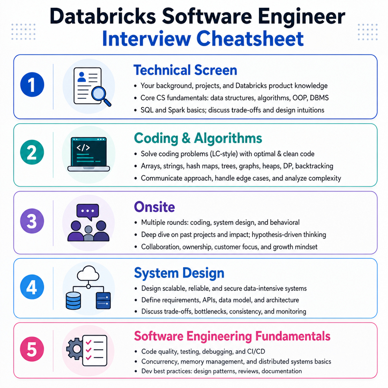
Focus most on Databricks production-system design—KV/WAL durability, concurrency, lakehouse metadata, and shuffle/skew—because you are 0 YOE, self-rated systems 3/5, and have no solved-system history. Merely review lower-priority coding variants like Tic-Tac-Toe engines, Fibonacci navigation, and RLE codecs; your Coding & Algorithms engagement is high with 44 views and 15 likes, and no extra coding subtopics were selected. Databricks-specific highlights are query-plan pruning/pushdown, lakehouse-style transaction metadata, and distributed query execution/shuffle trade-offs. With one month until the interview, budget about 70 minutes per full cheatsheet pass, then spend most remaining practice time implementing timed coding problems and explaining system trade-offs aloud.

Technical Screen — 16 min

Coding & Algorithms

• Sliding Window Counters And Rate Limiting — covered in depth under Onsite below.

• Snapshot Iterators And Versioned Sets — covered in depth under Onsite below.

• CIDR IPv4 Firewall Matching — covered in depth under Onsite below.

• Revenue Referral Aggregation And Ranking — covered in depth under Onsite below.

Onsite — 51 min

System Design

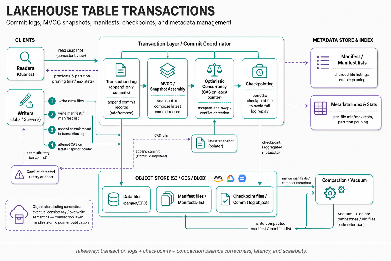
Focus area — Databricks-specific addendum: understand transaction logs, table metadata, snapshots, compaction, and optimistic commits at a high level.

What's being tested

Interviewers are probing your understanding of how a lakehouse implements ACID semantics, metadata management, and concurrent access at scale. Expect to demonstrate knowledge of transaction logs, snapshot isolation/MVCC, commit protocols, metadata indexing/pruning, and tradeoffs between consistency, latency, and scalability. Databricks cares because robust table transactions and compact metadata are central to correctness, query performance, and multi-tenant reliability on object stores.

Core knowledge

• Delta Lake, Apache Iceberg, Apache Hudi — three common lakehouse formats that implement transaction/metadata layers on object stores; compare by metadata size, management model, and compaction strategies.

• Transaction log / commit record — an append-only sequence that records file-level actions (add/remove); clients read the latest commit to assemble a table snapshot; logs must be atomic and idempotent.

• Multi-Version Concurrency Control (MVCC) and Snapshot Isolation — readers see a consistent snapshot created at commit-time; writers produce a new snapshot by composing previous metadata plus changes; prevents read-write conflicts without locking readers.

• Optimistic concurrency — writers compute new snapshot and attempt to atomically publish; conflict detection is typically a compare-and-swap on the latest log/manifest pointer; rollbacks require compensating commits or tombstones.

• Manifest/manifest lists — metadata files (manifests) list data files for a snapshot; manifest lists scale metadata by sharding file listings and enable pruning during query planning.

• Compaction and vacuuming — merging small metadata or data files improves query planning and IO; aggressive compaction reduces metadata files but increases CPU and temporary storage usage.

• Checkpointing — periodic snapshots of in-memory/aggregated metadata produce a single checkpoint file so recovering the latest state avoids replaying the entire log; checkpoint frequency trades off recovery time vs write amplification.

• Metadata pruning & partition pruning — push predicate filters into metadata level to avoid listing large numbers of files; maintain per-file min/max stats (e.g., min_ts, max_ts) for efficient pruning.

• Consistency on object stores (S3/GCS) — object stores have eventual consistency semantics for listing/overwrite historically; transaction layers use atomic rename/manifest pointers or a consensus service to guarantee linearizable commits.

• Garbage collection / retention policy — deleted files remain referenced by older snapshots until TTL; retention windows must balance time-travel requirements vs storage cost; implement safe GC by ensuring no active transaction references removed objects.

• Performance numbers & thresholds — metadata operations (e.g., listing 100k files) dominate planning; formats target keeping manifest size < ~100k entries for plan-time performance; beyond ~1M entries, push to partition-level indices or catalog services.

• Distributed commit coordination — small teams use file-atomic operations; large deployments use consensus (e.g., Raft/Paxos) or a centralized metastore for strong coordination and leader-based commit ordering.

Tip: design metadata APIs for idempotent retries (idempotency-key) and fast conflict detection to simplify client retry logic.

Worked example — designing a transactional metadata layer for a table

Frame the problem: clarify required guarantees (atomic commit? snapshot isolation? time-travel TTL?), expected workload (many small file writers vs large batch writes), and storage backend (S3/HDFS). A strong candidate outlines three pillars: the commit protocol (how a writer publishes a new snapshot), the metadata organization (log, checkpoints, manifests), and the cleanup/compaction lifecycle. Describe using an append-only transaction log where each commit writes a new JSON/Parquet entry and an atomic pointer update (or consensus-backed record) publishes the new head; readers reconstruct snapshots by reading the latest checkpoint plus subsequent commits. Call out a tradeoff: frequent checkpointing reduces recovery time but increases write amplification and storage I/O. Close by saying: if time permits, discuss implementing optimistic concurrency with per-commit version checks, instrumentation for commit conflicts, and a background compaction/vacuum service to collapse small files and prune old snapshots.

A second angle — supporting high-concurrency streaming writers

Reframe: now many writers concurrently append micro-batches to the same table (stream ingestion). Emphasize per-writer local buffering and aggregation to reduce commit rate, and use optimistic commits with conflict detection on path (file-level) rather than whole-table. Introduce a lightweight leasing or leader-election (short-duration leader) to serialize commits when conflict rates spike, trading some latency for lower aborts. Explain manifest sharding by partition (e.g., date-hour) so parallel commits touch disjoint manifests, minimizing contention. Also mention backpressure: if commit conflicts rise, throttle upstream producers or increase batch sizes to reduce throughput pressure on metadata.

Common pitfalls

Pitfall: assuming object-store PUTs are atomic and listing is strongly consistent.

Many designs incorrectly treat object-store listings as instantaneous; on S3 you must avoid protocols that rely on immediate list visibility and instead use atomic pointer files, checkpoints, or a consensus service for head updates.

Pitfall: designing metadata that grows linearly without compaction.

Naive logs/manifests will degrade query planning as commits accumulate; failing to implement checkpointing/compaction leads to O(N) recovery and O(N) planning cost, where N is number of commits.

Pitfall: hiding retention/GC tradeoffs from users.

Automatic deletion of old files to save cost can break reproducibility/time-travel; surface retention policies and offer safe GC that verifies no active snapshot references exist.

Connections

Implementing table transactions and metadata naturally leads to adjacent topics: catalog services (e.g., Hive Metastore or a custom catalog for fast metadata lookup) and query planning/optimizer integration (how metadata pruning feeds statistics). Interviewers may also pivot into distributed consensus (e.g., Raft) when discussing strong commit ordering or into storage-layout optimization (formatting, file sizes, columnar vs row).

Further reading

• Delta Lake Transaction Log (Databricks) — concise overview of commit log, checkpoints, and time travel.

• Apache Iceberg Design — explains manifest lists, snapshotting, and partition-evolution with strong scalability focus.

Practice questions

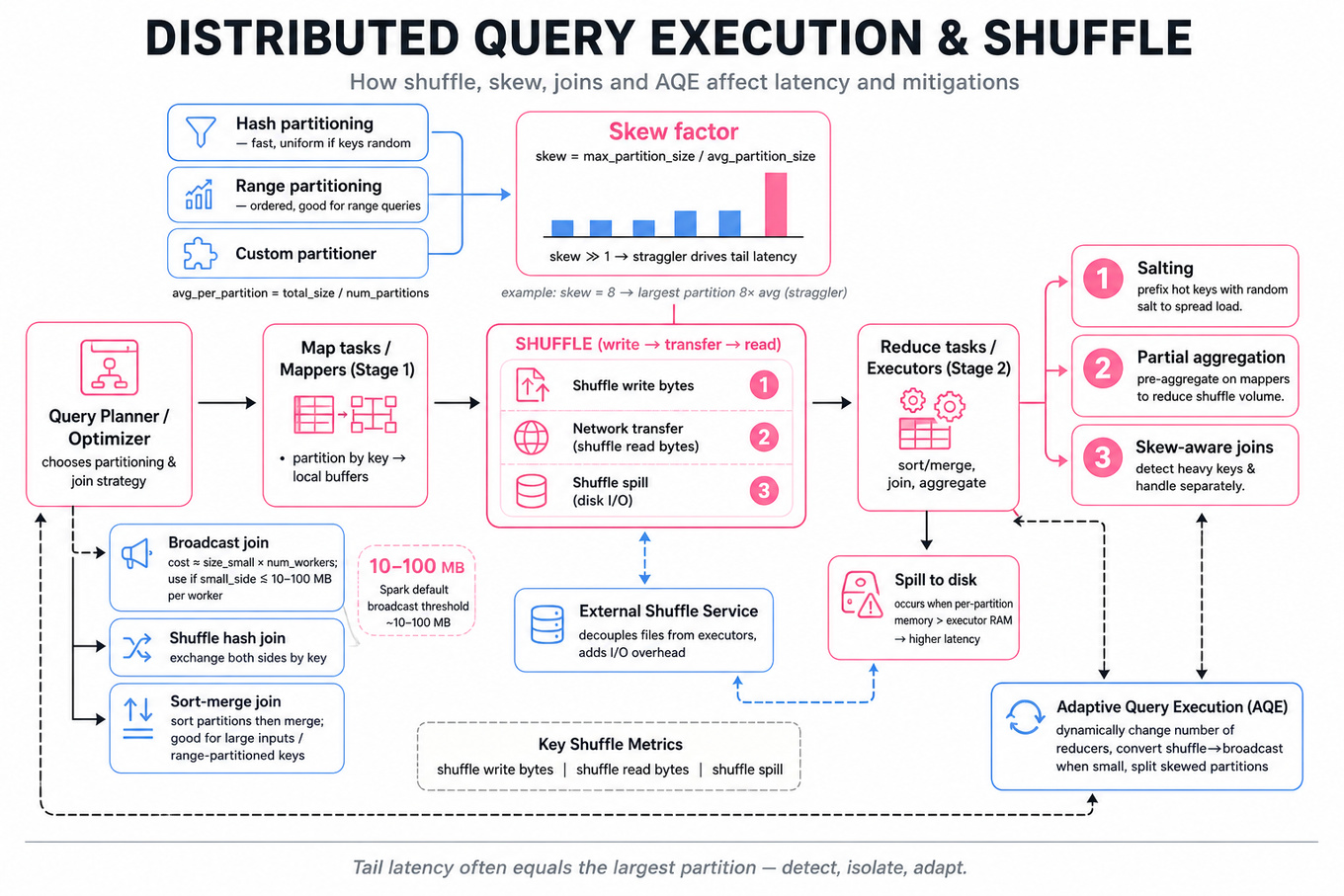
Focus area — Databricks-specific addendum: practice explaining partitioning, shuffle cost, stragglers, skew mitigation, and fault recovery.

What's being tested

Interviewers probe your practical understanding of distributed query execution: how shuffle moves data between stages, why skew breaks parallelism, and which execution strategies (partitioning, join algorithms, spilling, broadcasting, and adaptive execution) reduce latency and cost. Databricks cares because efficient shuffles directly affect job tail latency, cluster utilization, and SLOs; you must show concrete tradeoffs, measurable metrics, and an actionable mitigation plan a backend engineer would implement or tune.

Core knowledge

• Shuffle: the network+disk phase that redistributes records by partition key between map and reduce tasks; cost dominated by bytes written, transferred, and read. Metrics: shuffle write bytes, shuffle read bytes, and shuffle spill.

• Partitioning strategies: hash partitioning (fast, uniform if keys random) vs range partitioning (ordered, good for range queries) vs custom partitioners; average per-partition size = total_size / num_partitions.

• Skew definition & metric: skew factor = max_partition_size / avg_partition_size; values ≫1 indicate bad skew. Tail latency often driven by single largest partition (straggler).

• Join algorithms: broadcast join (send small table to all workers, cost ~size_small * num_workers), shuffle hash join (hash & exchange both sides), sort-merge join (sort partitions then merge; good for large inputs and range-partitioned keys).

• Thresholds & heuristics: broadcasting practical when the small side is ≲ tens of MBs per worker (Spark default ~10–100 MB); otherwise prefer shuffle join. When per-partition memory > available executor RAM, expect spill-to-disk and higher latency.

• Spill and external shuffle: when in-memory buffers exceed memory, tasks spill to disk; external shuffle services (e.g., Spark External Shuffle Service) decouple shuffle file lifetime from executors but add I/O and management complexity.

• Skew mitigation techniques: salting (prefix keys with random salt to spread hot keys), partial aggregation (pre-aggregate on mappers), skew-aware joins (detect heavy keys and handle separately), and increasing partitions (finer parallelism but higher overhead).

• Adaptive Query Execution (AQE): runtime adjustments based on observed metrics — e.g., dynamically change number of reducers, convert shuffle join to broadcast join when small, or split skewed partition into multiple tasks.

• I/O and network tradeoffs: increasing partitions reduces per-task memory but raises metadata and RPC overhead; salting increases shuffle volume by factor ≈ average_salt_count.

• Speculation & retries: enable speculative execution to mitigate transient stragglers, but beware job duplication amplifying load on hot partitions.

• Instrumentation to act: know where to read shuffleReadMetrics, shuffleWriteMetrics, executor logs, per-task CPU/wall time, and OS-level metrics (disk IO, network bandwidth) to attribute bottlenecks.

• Complexity and cost model: model job time ≈ max_over_partitions(read + compute + write + network) where network ≈ shuffle_bytes / network_bandwidth; optimizations should reduce either bytes or critical path.

Worked example — "Explain how shuffle works and how to mitigate skew"

First 30s: ask clarifying Qs — input sizes per relation, key cardinality and distribution (Zipfian?), available executor memory, and whether joins are equi-joins or range joins. Frame goal: minimize job p99 latency and network I/O.

Answer skeleton:

1. Describe shuffle phases: partitioning at mappers, writing local files, block transfer, and reduce-side read/merge.

2. Show cost model: per-partition bytes and latency dominated by largest partition; compute skew factor.

3. Present mitigation options in order: broadcast if small, pre-aggregate, increase partitions, salting or skew-aware split, AQE, and speculative execution.

4. Implementation notes: tune spark.sql.shuffle.partitions, broadcast threshold, and monitor shuffleReadBytes/shuffleWriteBytes.

Tradeoff to call out: salting reduces straggler risk but multiplies shuffle bytes and complicates correctness (requires un-salting post-aggregation). Communicate measurable criteria: apply salting only when skew factor > X (e.g., 10) and heavy-key bytes exceed single-task memory.

Close: propose an experiment plan — run instrumented job with varying spark.sql.shuffle.partitions, enable AQE, and compare p50/p95/p99 and shuffle bytes; say "if more time, I'd prototype salting and measure end-to-end cost vs benefit."

A second angle — "Detecting and fixing skew at runtime on production jobs"

Frame: you cannot change job code easily; you can observe metrics and apply runtime fixes. Strategy: detect hot partitions via shuffleReadMetrics and task durations, then (1) if small table detected, trigger broadcast dynamically; (2) if skewed keys present, use AQE to split large partitions into multiple reducers; (3) enable speculative tasks for the straggler. Emphasize low-risk fixes first (tuning partition count, enabling AQE/speculation) before code-intrusive solutions (salting). Highlight tradeoffs: AQE relies on accurate sampling and may not catch transient spikes; speculative execution duplicates work and can worsen load if the system is I/O-bound.

Common pitfalls

Pitfall: assuming uniform key distribution — candidates often propose hash partitioning without checking for Zipfian/long-tail distributions; always inspect key cardinality and frequency histogram.

Pitfall: recommending "just increase partitions" without cost modeling — more partitions can reduce per-task memory but increases small-file, metadata, and network overhead, sometimes worsening latency.

Pitfall: suggesting broadcast join blindly — if the broadcasted dataset exceeds memory or the cluster has many executors, broadcasting increases GC pressure and may OOM workers; prefer runtime checks and AQE to flip strategies.

Connections

• Query optimizers and cost-based optimization (how statistics enable broadcast vs shuffle decisions).

• Task scheduling and speculative execution, because skew creates stragglers that schedulers may mitigate or exacerbate.

• Storage and I/O systems (local SSDs, remote shuffle service) since disk throughput and latency often dominate spilled-shuffle cost.

Further reading

• Spark: The Definitive Guide — chapters on shuffle, joins, and tuning.

• Databricks blog — Adaptive Query Execution in Spark — practical AQE techniques and tradeoffs.

Practice questions

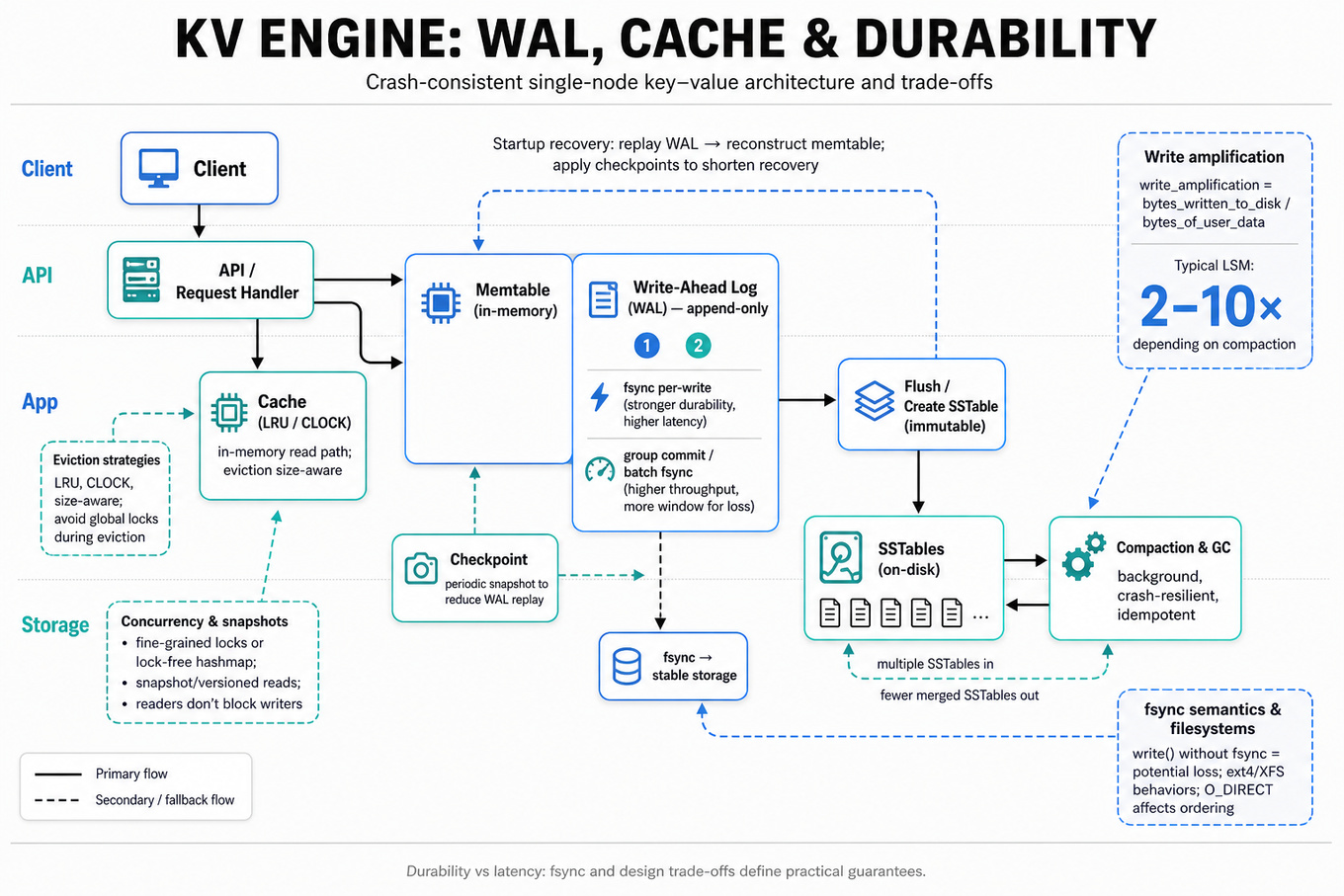
Focus area — Databricks values storage correctness; 0 YOE and no solved system-design history make WAL trade-offs worth emphasizing.

What's being tested

Interviewers probe your ability to design a crash-consistent, single-node key–value engine that balances latency, durability, and memory/disk trade-offs while being implementable by an engineer in a coding interview. They expect clear scoping questions, a layered design (API, in-memory structures, on-disk layout, recovery, concurrency), and justification of trade-offs such as synchronous durability versus throughput. Databricks cares because production tooling (local storage engines, caching layers, metadata services) must be correct under crashes and perform predictably.

Core knowledge

• Write-Ahead Log (WAL): append-only log of mutations; guarantees durability if writes are synced to stable storage before acknowledging. Group commit reduces fsync cost; per-write fsync gives stronger durability but higher latency.

• memtable and SSTable: common LSM approach uses an in-memory memtable for fast writes and immutable on-disk SSTables written by compaction; provides high write throughput at cost of read amplification.

• B-tree vs LSM-tree tradeoff: B-tree gives lower read amplification and predictable range scans; LSM-tree optimizes write throughput and sequential IO on disk; pick by read/write ratio and latency targets.

• fsync semantics and filesystems: fsync on ext4/XFS vs O_DIRECT affect durability and ordering; understand that write() without fsync risks data loss on crash. fsync latency dominates small-write throughput.

• Write amplification formula: write_amplification = bytes_written_to_disk / bytes_of_user_data; compaction increases amplification — quantify (LSM often 2–10x depending on compaction).

• Compaction and GC: background compaction merges SSTables; tune compaction concurrency to limit IO interference and reduce read amplification; ensure compaction is crash-resilient and idempotent.

• Atomicity & Recovery: recovery replays WAL then applies any partially-written files; checkpoints reduce recovery time by persisting a consistent on-disk snapshot of in-memory state.

• Concurrency control: use fine-grained locks or lock-free concurrent hashmaps for in-memory access; readers should avoid blocking writers (snapshot isolation or versioned reads).

• Eviction strategies: LRU, CLOCK, or size-aware eviction for an in-memory cache; consider entry sizes and avoid heavy global locks during eviction.

• Persistence modes for caches: write-through (sync to WAL before ack) vs write-back (ack then persist later) — trade latency vs data loss risk.

• Atomic replace / rename: use atomic rename() for installing new SSTables/checkpoints to avoid partial files being picked up during recovery.

• Testing and metrics: measure p99 latency, throughput, and recovery time; fuzz crashes and power-fail to validate durability guarantees.

Worked example — "Design a key-value store"

Start by clarifying requirements: expected dataset size, read/write ratio, latency SLOs (p99), single-writer or concurrent-writers, durability level (ack after WAL fsync or async). Declare assumptions (single-node, dataset up to ~100GB, memory budget 8–32GB).

Organize the answer into pillars: (1) API and consistency model (simple get/put/delete, optional snapshots); (2) in-memory front (concurrent hash map + memtable) and background flush; (3) on-disk format (append-only WAL, immutable SSTables with checksums); (4) recovery and compaction; (5) concurrency and durability knobs.

Detail one tradeoff: choose LSM-tree with WAL+memtable if writes dominate — justify that sequential IO makes fsync grouping effective; if low-latency reads and range scans dominate, argue for a B-tree style approach. Explicitly call out fsync cost and propose group commit / configurable durability levels.

Close by describing tests and next steps: "If I had more time I'd sketch on-disk block layout (checksums, footer), show pseudocode for recovery and WAL truncation, and propose benchmarks (YCSB) plus crash-fuzz tests."

A second angle — "Design a single-node persistent in-memory cache"

Here the emphasis shifts to strict in-memory performance with optional persistence. Start by clarifying durability semantics: checkpointing vs synchronous WAL. Design pillars: memory-efficient in-memory store (sharded concurrent hashmap), eviction policy tuned to object size and access frequency (LRU or segmented LRU), and a persistence layer that snapshots memory periodically while writing an incremental WAL for recent mutations.

Key differences: minimize write path latency — prefer async persistence (write-back) with a small window of potential data loss, and use background threads to do checkpointing/compaction. Also, reduce contention via sharding and lock-striping; in high-throughput scenarios, measure latency impact of checkpoint fsync and stagger checkpoint start times. For small objects, serialization/deserialization cost matters — use zero-copy or memory arenas when possible.

Common pitfalls

Pitfall: Assuming write() implies durability. Many candidates forget that write() without fsync can lose data on crash; always state when you require fsync or opt for configurable durability.

Pitfall: Sketching a single global lock for all operations. That simplifies correctness but kills throughput; prefer sharded locks, lock-free structures, or read-copy-update/snapshots for readers.

Pitfall: Ignoring recovery complexity. Saying "replay WAL" without addressing partial writes, checksums, and atomic SSTable installation misses correctness; describe atomic file replacement and WAL truncation.

Connections

Interviewers may pivot to distributed versions (introduce consensus via Raft/Paxos for multi-node durability), or to storage-layer details (block-device behavior, fsync latency, O_DIRECT). They might also ask about benchmarking (YCSB) or profiling hotspots (perf, flamegraphs).

Further reading

• Designing Data-Intensive Applications — Martin Kleppmann — deep coverage of storage engines, LSM vs B-tree tradeoffs.

• RocksDB GitHub — production LSM implementation to study memtable, WAL, compaction strategies.

• PostgreSQL WAL documentation — concrete explanation of WAL durability semantics.

Practice questions

Important onsite backend theme, but base coverage is enough without a special requirement calling it out.

What's being tested

Interviewers are probing your ability to design robust asynchronous services that tolerate network failures using correct idempotency and retry strategies while preserving correctness, auditability, and performance. Expect to justify tradeoffs between at-least-once vs exactly-once behaviors, pick storage and deduplication patterns, and describe operational controls (timeouts, backoff, metrics). Databricks values systems that remain correct under partial failure and that make clear, testable guarantees a software engineer can implement and maintain.

Core knowledge

• Idempotency — guarantee that repeating the same operation has the same effect; implement via an idempotency key (client-generated or server-generated) stored with outcome and TTL to deduplicate retries atomically.

• At-least-once vs exactly-once — at-least-once is simpler (retries may duplicate) while exactly-once requires coordination (dedup stores, distributed locks, or transactional sinks) and costs latency and complexity.

• Deduplication store patterns — use a single-row unique constraint in Postgres or a write-once record in Redis/Cassandra to record (idempotency_key, status, result); keep TTL to bound storage growth and support eventual GC.

• Retry policies & backoff — prefer exponential backoff with jitter to avoid thundering herds; cap retries and expose a failure mode to callers after N attempts. Quantify: start 100–200ms, double to a max ~5–10s.

• Synchronous vs asynchronous flows — synchronous (blocking) authorization provides immediate result but ties up clients; asynchronous (webhook, polling, callback) scales better for slow or multi-hop operations like external authorization.

• Compensating actions & reversals — for non-idempotent side effects (payments, stock reservation), model operations as two-phase: tentatively reserve then commit/settle, or create a compensating transaction (reversal) when downstream fails.

• Message delivery semantics — with Kafka/SQS expect at-least-once delivery; design consumers to be idempotent or use an exactly-once stream processor (e.g., Kafka Streams with EOS) when necessary.

• Ordering and causality — if order matters, use partitioning keys and monotonic offsets; for multi-participant operations, use logical timestamps or vector clocks to reason about concurrent retries and deletions.

• Durability and audit — persist the original request, idempotency key, response, and timeline (timestamps) to support reconciliation, dispute resolution, and retries. Use append-only logs for audit trails.

• Performance tradeoffs — deduplication lookups add latency (one extra read); choose read-before-write vs conditional write (INSERT ... ON CONFLICT DO NOTHING) depending on load: conditional writes scale better under high contention.

• Failure modes to test — network timeouts, duplicate client retries, partial downstream success, and long-tail latency spikes (p99 behaviour). Define SLAs: e.g., respond within 500ms for sync paths, otherwise escalate to async.

• Security and id generation — prefer collision-resistant ids (UUIDv4 or client nonce with HMAC) as idempotency keys; authenticate and bind keys to client credentials to prevent replay across accounts.

Worked example — Design a Visa-Style Card Payment Processing System

First 30 seconds: clarify scope (merchant-side acquirer vs global network), required latency for authorization, failure semantics (is double-charge acceptable?), and which parties can retry (merchant, gateway, issuer). State assumptions: we design an acquirer gateway handling authorizations and routing to issuers, with a requirement to avoid duplicate captures.

Skeleton pillars: (1) API & idempotency: require client-supplied idempotency_key per payment attempt and store (key, status, response) atomically; (2) Routing & async authorization: send authorization to issuer synchronously with a bounded timeout, else mark as PENDING and enqueue for async retry; (3) Settlement & ledger: an append-only settlement ledger records captures and reversals, with unique constraints to prevent duplicate entries; (4) Reconciliation & audit: background jobs reconcile pending states with issuers and emit compensating transactions for timeouts.

One tradeoff to flag: synchronous blocking gives merchant immediate truth but creates load and failures on issuer slow paths; asynchronous decouples latency but complicates customer UX and requires clear guarantees (e.g., eventual confirmation within X minutes). Implementation detail: use INSERT ... ON CONFLICT to create idempotency records atomically and return stored response if conflict occurs.

Close by stating next steps: if more time, add fraud filtering pipeline, a test harness to simulate partial issuer failures, and dashboards for p99 latency, retry counts, and reconciliation gaps.

A second angle — Design Chat APIs, Storage, and Message Flows

Chat emphasizes ordered, low-latency delivery and offline recovery, so idempotency focuses on message deduplication and reconnection correctness. Use client-generated monotonic message_id or UUID plus a send-sequence per conversation; server stores (conversation_id, message_id) to reject duplicates. For deletions and edits, model operations as idempotent commands with tombstones and causal metadata so offline clients converge (apply ops in sequence or use CRDTs for idempotent merge). Retries: clients should retry sends to server until acknowledged, server must be able to reply with the canonical message id/result to any duplicate send. The core concept—protecting side effects from duplicate retries—remains identical, but constraints (ordering, per-conversation partitioning, reconnect reconciliation) change data model and storage choices.

Common pitfalls

Pitfall: Treating retries purely as a client problem.

Many engineers assume client retries alone solve transient failures. In reality the server must detect duplicates (idempotency store) and return the prior result; otherwise clients will see inconsistent outcomes and operators face reconciliation headaches.

Pitfall: Over-engineering exactly-once when at-least-once suffices.

Chasing full exactly-once semantics across multiple systems often costs latency and complexity; prefer idempotent consumer/producer patterns and compensating transactions unless business correctness absolutely requires atomic cross-system commit.

Pitfall: Forgetting TTLs and GC for idempotency records.

Keeping deduplication records forever prevents replays but creates unbounded storage. Define an idempotency window aligned with business semantics (e.g., 24–72 hours) and a safe GC policy to reclaim space.

Connections

Interviewers may pivot to distributed transactions / two-phase commit, event sourcing / CQRS, or observability (tracing retries end-to-end). Be ready to discuss how idempotency integrates with monitoring (retry_count, duplicate_rate, reconciliation lag).

Further reading

• Designing Data-Intensive Applications — Martin Kleppmann — strong background on consistency, ordering, and deduplication patterns.

• Stripe: Idempotency Keys — practical implementation patterns and tradeoffs for payment systems.

Practice questions

Software Engineering Fundamentals

Focus area — Databricks-specific data-engineering signal; your 11 SE fundamentals views make this a valuable differentiator.

What's being tested

Two core skills: implementing column pruning and filter pushdown on a query-plan tree, and writing correct, efficient tree rewrites. Interviewers check recursive AST traversal, tracking required columns and predicates across Scan, Project, Filter, and Join nodes, plus sound handling of expression lineage and semantics.

Patterns & templates

• Bottom-up recursion: compute required columns for each node from its parent, revisit children with that set; linear time O(nodes) for fixed-size expressions.

• Predicate classification: split predicates into pushable (refer only to one child) and residual; push pushables down early to reduce rows.

• Column projection: at Scan emit only needed physical columns; at Project rewrite expressions to map child columns, prune unused projections.

• Join handling: push predicates that reference only one side into that side; predicates referencing both become join conditions. Handle outer joins conservatively.

• Expression substitution: maintain a mapping from parent output to child expressions for safe rewrite; avoid re-evaluating complex expressions.

• Immutability & CAS: return new nodes (functional updates) so rewrites are testable; memoize visited nodes to avoid exponential work.

Common pitfalls

Pitfall: Pushing a predicate that references columns produced by a Project without rewriting to the underlying Scan names — causes invalid plans.

Pitfall: Ignoring NULL semantics on outer joins and pushing predicates that change result cardinality.

Pitfall: Over-pruning columns used inside non-project side-effects (e.g., EXISTS, ORDER BY expressions) — leads to incorrect answers.

Practice these

The practice cards below cover the canonical variants — solve all of them and time yourself.

Practice questions

Coding & Algorithms

Core Databricks-style coding pattern; 3/5 coding self-rating and no solved history keep this at full practice depth.

What's being tested

These problems test designing and implementing sliding window counters for real-time per-key aggregation and rate limiting: correct time-window semantics, efficient per-key state, memory/CPU tradeoffs, and concurrency. Interviewers want to see clear assumptions about clock skew, event ordering, and cleanup/eviction strategies.

Patterns & templates

• Time-bucket counter — keep an array of B buckets (width = window/B); O(1) update, O(B) memory per key; rotate buckets on time tick.

• Exact timestamp window — store recent event timestamps in a deque; pop old entries, count remaining; O(k) memory (k = events in window).

• Token bucket — use tokens and refill rate to allow bursts while enforcing long-term rate; constant-time checks and updates per request.

• Leaky bucket — model as a drain-rate queue for smoothing; implement with last-timestamp and accumulated state, O(1) state per key.

• Per-key sharding + ConcurrentHashMap — store state per IP, shard by hash to avoid global locks; consider lock striping for atomic updates.

• Eviction/TTL — run background sweep or use TTL heap to remove idle keys; avoid unbounded growth when keys ≫ active window.

• Clock handling — use monotonic now() for deltas; convert timestamps to bucket indices deterministically to handle skew.

Common pitfalls

Pitfall: Using a fixed-window counter causes boundary burstiness — two windows can be abused to double rate across the boundary.

Pitfall: Forgetting eviction leads to memory leak when attackers create many unique keys; add TTL or LRU cleanup.

Pitfall: Doing per-request global locks kills throughput; use per-key atomic updates or lock striping instead.

Practice these

The practice cards below cover the canonical variants — solve all of them and time yourself.

Practice questions

No weak flag, but snapshot semantics are subtle enough to practice beyond a skim.

What's being tested

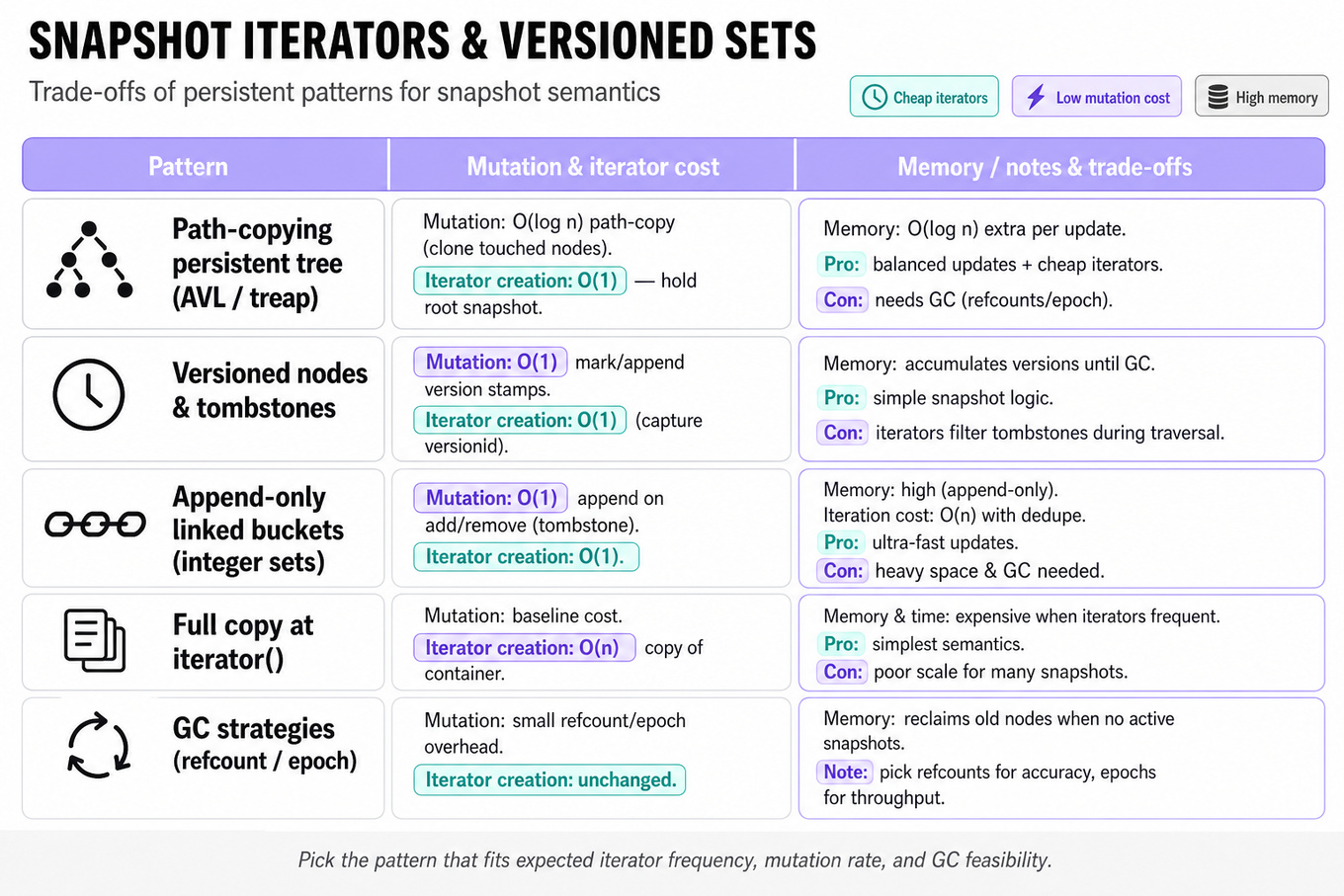
Candidates must demonstrate design and implementation of snapshot semantics over a mutable set, showing mastery of persistent data structures, iterator stability, and complexity trade-offs. Interviewers probe whether you can provide iterators that reflect a point-in-time view while keeping add()/remove() fast and memory usage bounded.

Patterns & templates

• Copy-on-write at mutation: on add()/remove() clone only touched nodes to give new version, enabling O(1) iterator creation and O(log n) mutation cost in trees.
• Versioned nodes with integer version stamps: iterator captures current versionId; nodes carry created/removed versions to decide visibility during traversal.
• Tombstone marking: mark removals with a tombstone timestamp instead of physical delete; iteration filters by snapshot versionId.
• Path-copying persistent tree (e.g., AVL/treap): O(log n) amortized updates, iterators cheaply reference root at snapshot creation.
• Append-only linked buckets for integer sets: add() appends, remove() appends tombstone; iterators scan and dedupe, trading space for O(1) updates.
• Garbage collection via refcounts or epoch-based reclamation: reclaim old nodes when no iterator references older versions.
• Complexity tradeoff template: iterator creation O(1) + iteration O(k) vs full-copy O(n) creation; pick based on expected concurrent iterators.

Common pitfalls

Pitfall: Returning a live iterator over the single backing container — it will reflect later mutations, violating snapshot semantics.

Pitfall: Naively full-copying at iterator() for correctness — correct but often fails memory/time constraints when iterators are frequent.

Pitfall: Forgetting to reclaim old versions — leads to unbounded memory growth; track active snapshots or use epoch GC.

Practice these

The practice cards below cover the canonical variants — solve all of them and time yourself.

Practice questions

Frequent implementation-heavy topic; normal weight because there are no completed solves despite high coding engagement.

What's being tested

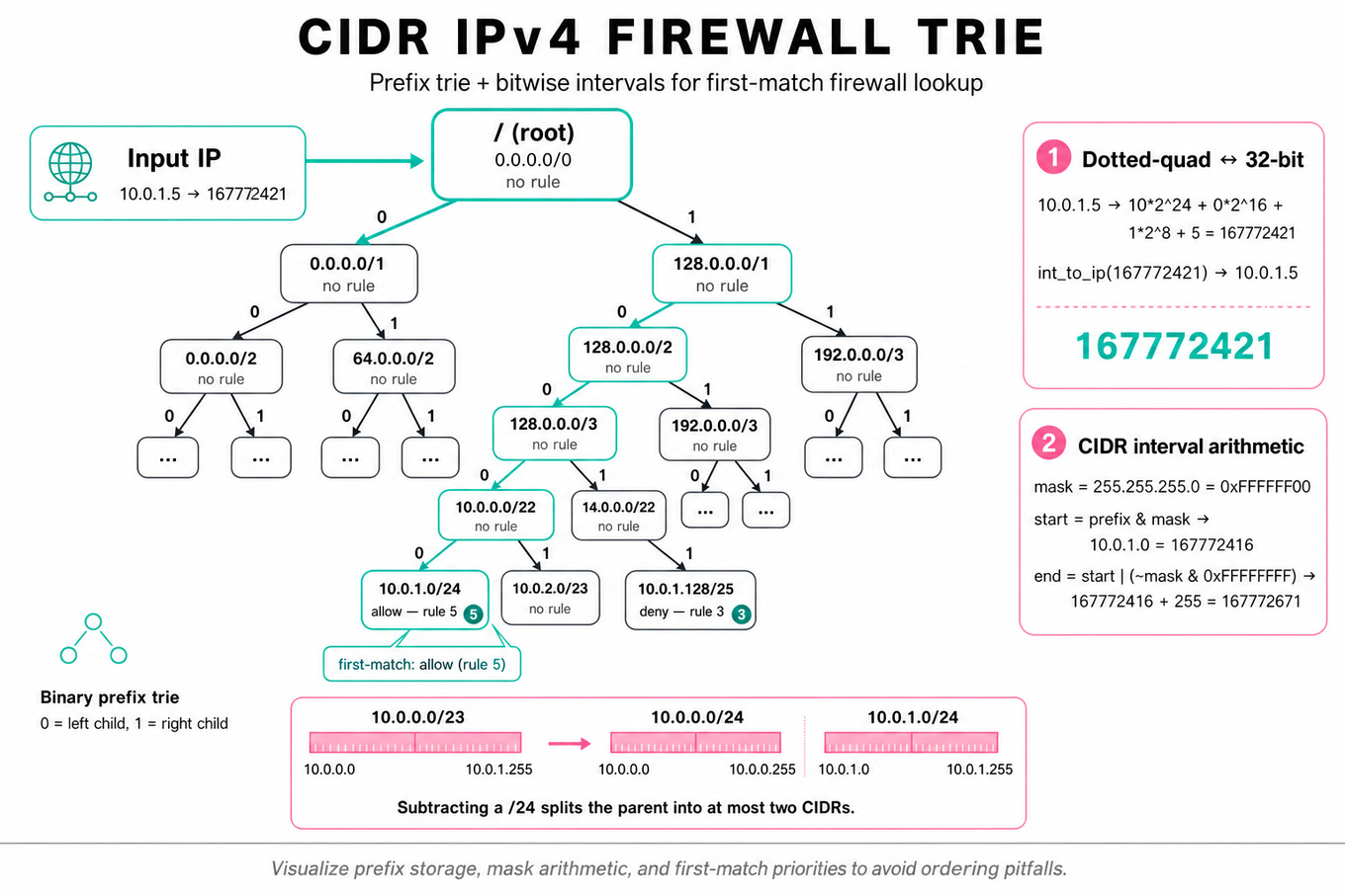
Candidates must demonstrate precise IPv4/CIDR arithmetic and set reasoning: convert between dotted quad and 32-bit integers, compute CIDR start/end, and test containment or overlap. Interviewers also probe algorithmic design for ordered first‑match firewall semantics and scalable lookup/update structures that keep matching low‑latency.

Patterns & templates

• Convert dotted-quad ↔ 32-bit with `ip_to_int` / `int_to_ip` and apply masks via (ip & mask) == (prefix & mask) for prefix containment.

• Represent a CIDR as a closed integer interval [start, end] using start = prefix & mask, end = start | (~mask & 0xFFFFFFFF).

• Prefix containment = single mask equality; overlap = interval intersection check with O(1) bit ops.

• Subtracting one CIDR from another: split into at most two smaller CIDRs using bitwise prefix shrink; repeated subtraction is interval-set difference.

• Ordered first-match firewall: evaluate rules sequentially until a match; for block queries, require full coverage of the block by an allowed rule (or absence of earlier deny).

• Use a prefix trie / binary radix tree for O(W) lookup where W ≤ 32; for N large, compress to a Patricia/radix trie to reduce memory and hops.

Tip: store rules at trie nodes with priority index to resolve first-match without linear scan.

Common pitfalls

Pitfall: confusing network vs broadcast addresses — treat CIDR ranges as inclusive [start, end] using 32-bit arithmetic.

Pitfall: assuming disjoint CIDRs — overlapping rules with ordering change semantics; always respect rule index priority.

Pitfall: using string parsing (regex) in hot path — convert once to ints/masks; runtime must be bitwise, not text-based.

Practice these

the practice cards below cover the canonical variants — solve all of them and time yourself

Practice questions

Maintain normal depth because dynamic aggregation and ranking are common coding-screen traps.

What's being tested

These problems test efficient aggregation of event streams into per-customer totals, plus selection/update of the k smallest totals under dynamic inputs. Interviewers probe algorithmic choices (selection vs. streaming top-k), data structures for incremental updates, and correctness under referral/tree propagation.

Patterns & templates

• Hash map for accumulator state: map customer -> total, O(1) amortized updates, size O(N); watch memory when N → millions.

• Max-heap of size k to maintain k smallest totals: push O(log k), keep heap size k, overall O(n log k) for one-pass selection.

• Quickselect for one-shot smallest-k selection: average O(n) time, O(1) extra space, unstable under frequent updates.

• Indexed priority queue / balanced BST for dynamic insert/update/delete with O(log n) per update when reads interleave writes.

• Euler tour + Fenwick tree (BIT) / segment tree to support subtree-sum updates and ancestor queries in O(log n) for referral-propagation problems.

• DFS/BFS to traverse referral graph for initial build or validation; detect cycles with white/gray/black visitation to enforce acyclic referrals.

• Stable tie-breaking: include deterministic secondary key (creation timestamp or id) to ensure reproducible ordering on equal revenues.

Common pitfalls

Pitfall: Using a simple sort for repeated queries — O(n log n) per query blows up when queries are frequent or state is streaming.

Pitfall: Not handling referral cycles — assume DAG only after explicitly validating inputs to avoid infinite propagation.

Pitfall: Updating all ancestors naively on every event — O(depth) per event can be O(n) worst-case; use subtree-indexed structures for scale.

Practice these

The practice cards below cover the canonical variants — solve all of them and time yourself.

Practice questions