DoorDash Data Scientist Interview Prep Guide

Technical Screen

Data Manipulation (SQL/Python)

• SQL — covered in depth under Onsite below.

• Window Functions — covered in depth under Onsite below.

Analytics & Experimentation

• A/B Testing — covered in depth under Onsite below.

• Causal Inference — covered in depth under Onsite below.

• Marketplace Metric Frameworks — covered in depth under Onsite below.

• Operational Delivery Quality Diagnostics — covered in depth under Onsite below.

• Marketplace Interference And Switchback Experiments — covered in depth under Onsite below.

• Unit Economics And Pricing Analytics — covered in depth under Onsite below.

Statistics & Math

• Statistical Power Analysis — covered in depth under Onsite below.

Onsite

Data Manipulation (SQL/Python)

What's being tested

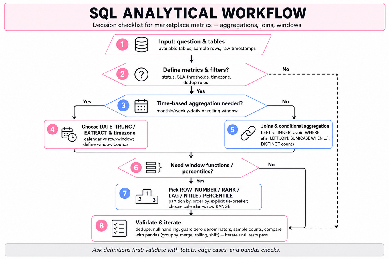
These questions test SQL analytical data manipulation for marketplace metrics: aggregating orders, joining customer/restaurant/event tables, grouping by time, ranking entities, and computing rates or percentiles. Interviewers are probing whether you can translate ambiguous DoorDash business definitions into correct SQL or Python logic with clean handling of timestamps, nulls, duplicates, and windowed metrics.

Patterns & templates

• Time-based aggregation — use `DATE_TRUNC`(`'month'`, `created_at`) or `EXTRACT` for monthly metrics; confirm timezone and order-status filters upfront.

• Conditional aggregation — compute rates with `SUM`(`CASE WHEN condition THEN 1 ELSE 0 END) * 1.0 / `COUNT`(*); guard against zero denominators.

• Entity ranking — use `ROW_NUMBER`, `RANK`, or `DENSE_RANK` with `PARTITION BY` for top customers, restaurants, or months; define tie-breaking explicitly.

• Windowed rolling metrics — use `AVG`, `SUM`, or `COUNT` over `ROWS BETWEEN` or date-range windows; distinguish row-count windows from calendar windows.

• Percentiles and quartiles — use `PERCENTILE_CONT`, `NTILE`(`4`), or `APPROX_PERCENTILE`; know whether the question needs exact thresholds or segmentation buckets.

• Event sequencing — use `LAG`, `LEAD`, and `ROW_NUMBER()` OVER (`PARTITION BY order_id ORDER BY event_ts`) to identify request flows and latest valid states.

• Python equivalent — map SQL patterns to `pandas`: `groupby`, `agg`, `merge`, `rank`, `rolling`, `quantile`, and `shift`; watch memory for large tables.

Common pitfalls

Pitfall: Counting rows instead of distinct orders or customers can inflate metrics after joins, especially with order-event or item-level tables.

Pitfall: Treating “late,” “cold,” or “completed” as obvious definitions without asking for SLA thresholds, cancellation handling, and timestamp source.

Pitfall: Using `WHERE` filters after a `LEFT JOIN` can silently turn it into an inner join and drop customers or restaurants with zero activity.

Practice these

The practice cards below cover the canonical variants — solve all of them and time yourself.

Practice questions

What's being tested

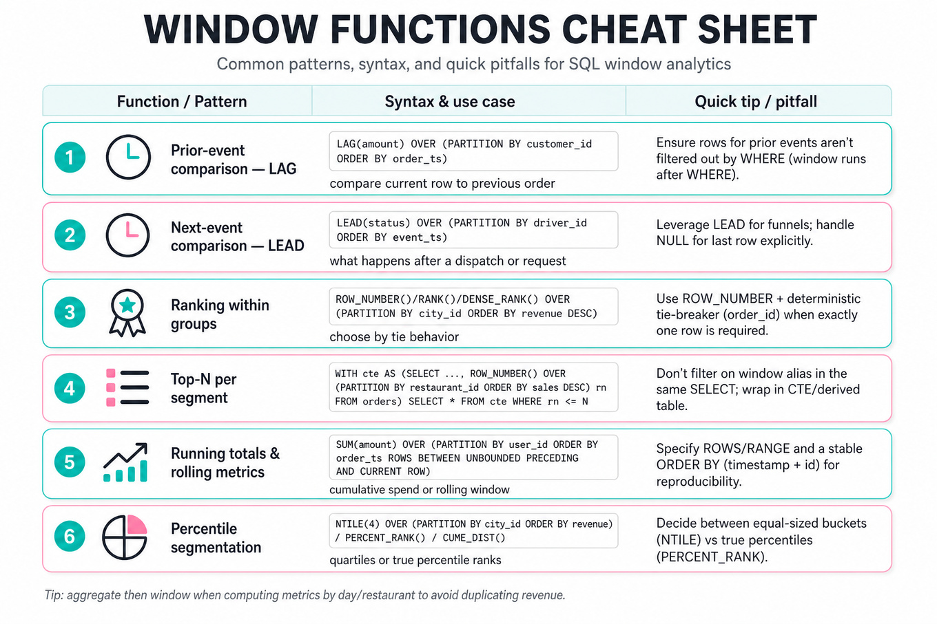
These problems test window-function analytics over customer, order, driver, restaurant, and city-level event data. You need to partition entities, order events in time, compare current rows to prior rows, rank within groups, and combine row-level windows with aggregations without losing analytical meaning.

Patterns & templates

• Prior-event comparison — use LAG(value) OVER (PARTITION BY customer_id ORDER BY order_ts) to compute spend changes, reorder gaps, or previous restaurant/city.

• Next-event comparison — use LEAD(status) OVER (...) when analyzing driver request sequences, acceptance funnels, or what happened after a dispatch attempt.

• Ranking within groups — use ROW_NUMBER, RANK, or DENSE_RANK with PARTITION BY city_id / restaurant_id; choose based on tie behavior.

• Top-N per segment — wrap window output in a CTE, then filter WHERE rn <= N; avoid filtering window aliases in the same SELECT.

• Running totals and rolling metrics — use SUM(amount) OVER (PARTITION BY user_id ORDER BY order_ts ROWS BETWEEN UNBOUNDED PRECEDING AND CURRENT ROW) for cumulative spend.

• Percentile segmentation — use NTILE(4), PERCENT_RANK, or CUME_DIST for quartiles; validate whether equal-sized buckets or true percentile thresholds are intended.

• Aggregate then window — first group to restaurant/day/customer level, then apply windows; mixing raw order rows with grouped metrics often duplicates revenue.

Common pitfalls

Pitfall: Using RANK when the interviewer expects exactly one row per group; use ROW_NUMBER with a deterministic tie-breaker like order_id.

Pitfall: Forgetting that window functions run after WHERE, so filtering dates or statuses too early can remove rows needed for prior-event comparisons.

Pitfall: Ordering only by date when multiple orders occur on the same day; include timestamp and stable IDs to make results reproducible.

Practice these

The practice cards below cover the canonical variants — solve all of them and time yourself.

Practice questions

Analytics & Experimentation

What's being tested

DoorDash A/B testing interviews probe whether you can design causal experiments in a two-sided marketplace where users, Dashers, merchants, time, and geography interact. The interviewer is looking for more than “split users 50/50 and compare conversion”; they want to see if you choose the right randomization unit, anticipate interference, define metrics that capture marketplace tradeoffs, and interpret noisy results without overclaiming. DoorDash cares because many product and algorithm changes affect supply-demand balance: batching, dispatch, Dasher modes, fees, promotions, and geo-targeted launches can improve one side of the marketplace while harming another. A strong Data Scientist answer combines experimental design, metric reasoning, power analysis, and causal interpretation under operational constraints.

Core knowledge

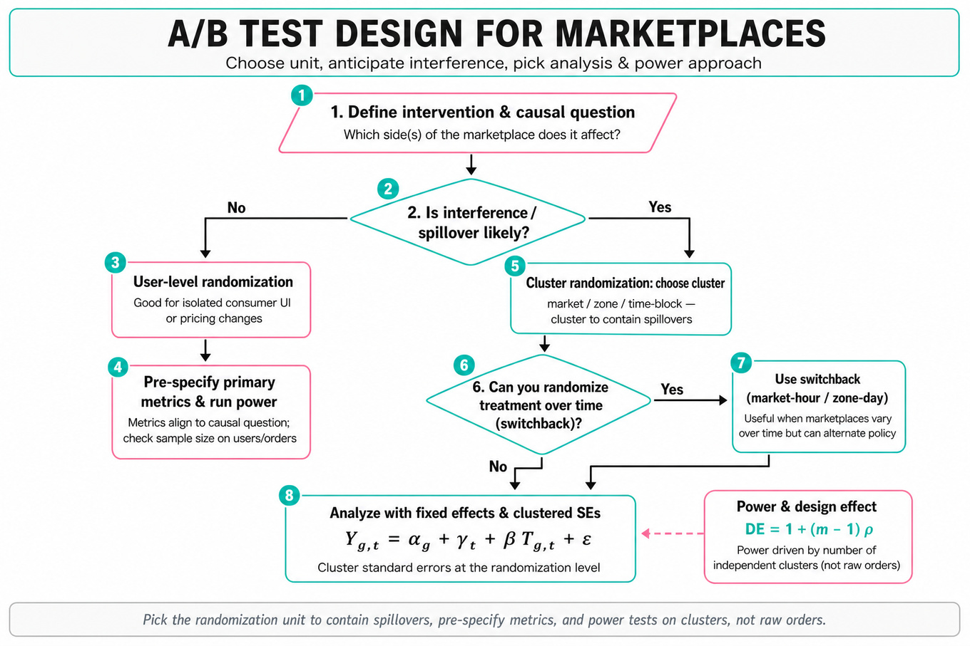
• Randomization unit is the first design decision. User-level randomization works for independent consumer UI changes, but marketplace interventions often need geo-level, time-level, or geo-time switchback randomization because one treated order can change Dasher availability, merchant wait time, and nearby customer experience.

• Interference / spillover violates the Stable Unit Treatment Value Assumption: one unit’s treatment changes another unit’s outcome. For DoorDash, batching, dispatch ranking, bicycle Dashers, and delivery radius changes can reallocate supply. If interference is likely, prefer cluster randomization by market, zone, or time block.

• Switchback experiments randomize treatment over time within a geography, commonly by market-hour or zone-day. They are useful when marketplace conditions vary heavily across markets but can tolerate alternating policies. Analyze with fixed effects such as market and time:
  $Y_{g,t}=\alpha_g+\gamma_t+\beta T_{g,t}+\epsilon_{g,t}$
  using clustered standard errors at the randomization level.

• Clustered designs reduce effective sample size. Power is driven by the number of independent clusters, not raw orders. The design effect is approximately:
  $DE = 1 + (m-1)\rho$
  where $m$ is cluster size and $\rho$ is intra-cluster correlation. Millions of orders can still be underpowered if randomized across only 10 markets.

• Primary metrics should align with the causal question and be chosen before launch. For revenue algorithms, candidates might define gross_order_value, contribution_profit, take_rate, or revenue_per_visitor; for logistics changes, use delivery_time, on_time_rate, dasher_utilization, cancellation_rate, and customer_retention.

• Guardrail metrics prevent local optimization. A batching algorithm may increase orders_per_dasher_hour but hurt ETA_accuracy, food quality, merchant wait, or NPS. A geo-targeted retention feature may improve D7_retention while increasing refunds or late deliveries.

• Marketplace metrics need segmentation. Always inspect treatment effects by market density, peak/off-peak, new vs existing customers, restaurant category, distance bands, Dasher mode, and supply-demand imbalance. Aggregates can hide Simpson’s paradox: high-density zones may benefit while suburban zones degrade.

• Power analysis should be stated in terms of minimum detectable effect. For a two-sample mean comparison:
  $n \approx \frac{2\sigma^2(z_{1-\alpha/2}+z_{1-\beta})^2}{\delta^2}$
  For proportions, replace $\sigma^2$ with $p(1-p)$. For clustered or switchback tests, inflate by design effect and use historical variance at the cluster-time level.

• CUPED / regression adjustment can improve precision when pre-period covariates predict outcomes. A common adjusted outcome is:
  $Y_i^{adj}=Y_i-\theta(X_i-\bar X)$
  where $X_i$ is a pre-treatment metric. This is especially useful for retention, order frequency, and revenue, but only if covariates are measured before treatment exposure.

• Intent-to-treat analysis is usually the default. Analyze users, orders, or clusters according to assigned treatment, not only those who complied. If there is noncompliance, report both ITT and possibly treatment-on-the-treated using assignment as an instrument, but be clear about assumptions.

• Sequential peeking inflates false positives. If stakeholders want daily reads, use pre-specified sequential methods such as alpha spending, group sequential boundaries, or Bayesian monitoring rules. Otherwise, communicate that interim dashboards are diagnostic, not decision-making.

• Novelty and learning effects matter for retention and logistics. A feature may spike short-term engagement but decay; a dispatch policy may need Dasher adaptation. For retention, inspect curves like D1, D7, D28, repeat order rate, and survival/hazard patterns rather than only a single endpoint.

Worked example

For Design and analyze a switchback experiment, a strong candidate would start by clarifying the intervention: “Is this a marketplace policy like batching, dispatch, or pricing that affects all orders in a zone during a time window?” They would then state that user-level randomization is probably inappropriate because treated and control orders compete for the same Dashers, causing interference. The answer skeleton should have four pillars: define the hypothesis and metrics, choose geo-time randomization, specify analysis, and cover power/operational risks.

A solid design would randomize treatment by zone × time_block, perhaps alternating 2- or 4-hour blocks, stratified by market, day of week, and peak/off-peak. The primary metric might be contribution_profit_per_order or delivery_time, with guardrails like cancellation_rate, merchant_wait_time, dasher_idle_time, and customer_rating. The analysis would regress the outcome on treatment with zone and time fixed effects, clustering standard errors at the zone or zone-time level depending on assignment and serial correlation. One tradeoff to flag explicitly is block length: shorter blocks increase sample size and balance, but risk carryover because Dashers, open deliveries, and customer demand do not reset instantly. The close should mention that with more time, you would test for pre-period balance, run placebo checks on pre-treatment periods, and examine heterogeneous effects by density and peak periods.

A second angle

For Analyze Retention Data for Geo-Targeted Feature Launch, the same causal logic applies, but the unit and outcome shift from operational time blocks to customer cohorts and retention curves. If the feature is launched only in selected geographies, the central risk is that treated markets differ systematically from control markets in seasonality, competition, promos, or customer mix. A strong answer would consider geo-matched controls, difference-in-differences, synthetic control, or staggered rollout analysis rather than a naive treated-vs-untreated comparison. The metric framing also changes: instead of immediate order-level outcomes, focus on D7_retention, D28_retention, repeat order frequency, cohort revenue, and whether retention gains persist after promotion or launch effects fade.

Common pitfalls

Pitfall: Treating every DoorDash experiment like independent user-level randomization.

The tempting answer is “randomly assign customers to treatment and control,” but that fails for dispatch, batching, Dasher supply, and marketplace policy changes. A better answer asks whether treatment changes the shared environment; if yes, move to geo, cluster, or switchback designs and analyze at the correct level.

Pitfall: Picking one success metric and ignoring marketplace tradeoffs.

Saying “we will launch if revenue increases” is incomplete because revenue can rise while delivery quality, Dasher earnings, merchant operations, or long-term retention decline. DoorDash DS interviews reward a balanced metric tree: one primary decision metric, several guardrails, and pre-specified segments where harm is plausible.

Pitfall: Overstating statistical significance without discussing power, variance, or clustering.

A candidate may quote a p-value from raw order-level data even though treatment was assigned by market-day. That usually understates uncertainty. The better response is to align the analysis unit with the randomization unit, use clustered standard errors or randomization inference, and explain whether the experiment had enough independent clusters to detect the desired effect.

Connections

Interviewers may pivot from A/B testing into causal inference, especially difference-in-differences, instrumental variables, synthetic controls, or matching for non-random rollouts. They may also connect to metric design, marketplace dynamics, ranking/recommender evaluation, or experimentation platform judgment such as sequential testing, heterogeneous treatment effects, and launch decision frameworks.

Further reading

• Trustworthy Online Controlled Experiments by Kohavi, Tang, and Xu — practical reference for online experiment design, metric selection, and decision errors.

• Causal Inference: The Mixtape by Scott Cunningham — accessible treatment of difference-in-differences, fixed effects, instruments, and quasi-experimental reasoning.

• Controlled experiments on the web: survey and practical guide, Kohavi et al. — classic paper on online experimentation pitfalls, metrics, and interpretation.

Practice questions

What's being tested

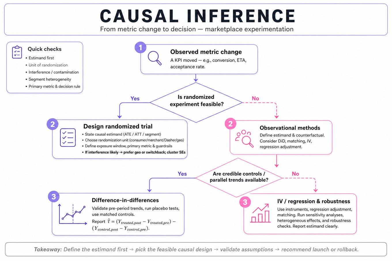
DoorDash causal inference interviews test whether you can move from “a metric changed” to “what caused it, how would we prove it, and what decision should we make?” The interviewer is probing for marketplace experimentation, counterfactual reasoning, metric design, and structured diagnosis across consumers, merchants, and Dashers. DoorDash cares because small operational changes—pay models, batching, merchant selection, grocery substitution flows, ETA promises—can shift multiple sides of the marketplace at once. A strong Data Scientist distinguishes correlation from causation, chooses the right unit of analysis, anticipates interference, and translates evidence into a launch or rollback recommendation.

Core knowledge

• Causal estimand comes before method. State whether you need the average treatment effect: $ATE = E[Y(1) - Y(0)]$, treatment effect on treated, local effect, or segment-specific effect. For DoorDash, effects often differ by market, daypart, merchant type, weather, and order distance.

• Randomized controlled trials are the gold standard when feasible. Define treatment, control, randomization unit, exposure window, primary metric, guardrails, and decision rule upfront. Common units include consumer, merchant, Dasher, delivery, store, or geo-market; the wrong unit can create contamination.

• Interference is central in marketplaces. One Dasher’s incentive treatment can affect untreated consumers through supply reallocation, batching, and ETA changes, violating SUTVA. If spillovers are likely, prefer geo-level randomization, switchback designs, or explicit network/market-level analysis over naive user-level randomization.

• Switchback experiments work well for operational levers that affect a market in real time, such as Dasher pay, dispatch logic, or batching. Randomize market-time blocks, for example city-hour or zone-daypart, and analyze with clustered standard errors. Watch for carryover effects if incentives alter Dasher positioning after the treatment block.

• Difference-in-differences estimates causal effects when randomization is unavailable:
  $\hat{\tau} = (Y_{treated,post} - Y_{treated,pre}) - (Y_{control,post} - Y_{control,pre})$
  Its key assumption is parallel trends. Validate with pre-period trend plots, placebo tests, and matched controls before trusting the estimate.

• Regression adjustment improves precision but does not magically remove bias. A model like $Y_i = \alpha + \beta T_i + \gamma X_i + \epsilon_i$ is credible when treatment assignment is as-good-as-random conditional on covariates. Include pre-treatment variables only; controlling for post-treatment mediators like actual delivery time can block part of the causal effect.

• Instrumental variables can help when treatment exposure is endogenous, but the bar is high. A valid instrument must affect the outcome only through treatment and be correlated with treatment. In delivery settings, examples are rare; randomized eligibility or phased rollout timing can sometimes serve, while raw distance or demand level usually fails exclusion restrictions.

• Metric hierarchy should separate primary outcomes, guardrails, and diagnostics. For late deliveries, primary metrics might be % deliveries > promised ETA + 10 min and consumer reorder rate; guardrails include Dasher earnings per active hour, merchant cancellations, refunds, and contribution profit. Diagnostics include pickup wait, travel time, batching rate, and prep-time error.

• Unit of analysis must match the causal question. For cold food complaints, order-level outcomes are natural, but consumer-level repeat behavior needs consumer aggregation. For merchant variety, treatment may be market-level because adding merchants changes the choice set for many consumers simultaneously.

• Power and minimum detectable effect should be discussed quantitatively. For a binary metric, approximate standard error is $\sqrt{p(1-p)/n}$. Rare events like cold-food complaints or grocery out-of-stock substitutions may need larger samples, longer tests, CUPED-style variance reduction, or a more frequent proxy metric.

• Heterogeneous treatment effects matter operationally but should be planned. Segment by market density, distance band, merchant category, new versus existing consumers, and daypart. Avoid fishing across dozens of cuts without correction; use pre-specified segments, hierarchical modeling, or false discovery rate controls when many comparisons are explored.

• Causal diagnosis is not only “run an experiment.” Start with metric validation, decomposition, temporal and geographic localization, cohort cuts, and funnel breakdowns. Then generate hypotheses and choose evidence: experiment if controllable, quasi-experiment if not, observational analysis for prioritization, and deep dives into logs or support labels as signal sources.

Worked example

For Diagnose and experiment to reduce late deliveries, a strong candidate would start by clarifying the definition of “late”: late relative to quoted ETA, promised delivery window, or actual food-ready time, and whether the business cares about order-level lateness, consumer experience, or merchant SLA. They would state assumptions such as “I’ll treat late delivery rate as the primary metric, with cancellation, refund rate, Dasher earnings, and reorder rate as guardrails.” The answer should be organized around four pillars: validate the metric and instrumentation, decompose the delivery lifecycle, identify causal hypotheses, and design experiments or quasi-experiments.

The diagnostic decomposition might split total delivery time into merchant prep time, Dasher assignment latency, travel-to-merchant, pickup wait, travel-to-consumer, and batching delay. The candidate should compare affected versus unaffected markets, dayparts, merchant types, weather conditions, and distance bands to isolate where the spike originates. If the leading hypothesis is inaccurate prep-time estimates, an experiment could adjust quoted prep-time buffers or merchant-facing prep prompts at the merchant or market level. If the hypothesis is Dasher supply shortage, a switchback test of incentives by zone-hour may be more appropriate than consumer-level randomization. A key tradeoff is that geo or switchback tests reduce interference but require more careful power calculations and clustered analysis. The close should be decision-oriented: “If the test reduces late rate without hurting Dasher earnings, merchant wait, or contribution margin, I’d recommend rollout; if I had more time, I’d estimate heterogeneous effects by market density and build a monitoring dashboard for recurrence.”

A second angle

For Define and Measure Merchant Variety's Impact on Consumers, the same causal toolkit applies, but the treatment is less like a single operational toggle and more like a change to the consumer choice set. The first task is defining merchant variety: count of available merchants, cuisine/category diversity, price-band coverage, distance-adjusted availability, or entropy of impressions/orders. A naive correlation between higher variety and higher order frequency is confounded because dense, high-demand markets naturally attract more merchants. Strong designs include geo-level expansion tests, phased merchant onboarding, matched market difference-in-differences, or synthetic controls for markets receiving new categories. The causal outcome should include consumer conversion and retention, but also merchant cannibalization, Dasher efficiency, and marketplace liquidity.

Common pitfalls

Pitfall: Treating correlation as causation.

A tempting answer is “markets with more merchants have higher retention, so variety improves retention.” That ignores demand density, income, urbanicity, marketing, and pre-existing consumer intent. A better answer states the counterfactual problem, proposes randomization or a quasi-experiment, and uses observational cuts only to prioritize hypotheses.

Pitfall: Optimizing one side of the marketplace in isolation.

For a Dasher compensation change, focusing only on delivery speed or acceptance rate is incomplete. Higher pay could improve fulfillment while hurting contribution margin, consumer fees, or merchant throughput; lower pay could preserve margin while creating supply shortages. DoorDash interviewers expect a balanced metric suite across consumers, merchants, Dashers, and business health.

Pitfall: Giving an experiment design without discussing interference and unit choice.

User-level A/B testing is often wrong for dispatch, pricing, selection, and operational levers because treated and control users share Dashers, merchants, and market capacity. Call out spillovers explicitly and choose market-level, store-level, cluster-level, or switchback randomization when marketplace equilibrium effects are likely.

Connections

Interviewers may pivot from causal inference into metric design, A/B testing and power analysis, root-cause analysis, marketplace dynamics, or ML model evaluation for ETA, ranking, and dispatch models. Be ready to discuss guardrail metrics, segmentation, novelty effects, multiple comparisons, and how offline model quality connects to online marketplace outcomes.

Further reading

• Mostly Harmless Econometrics — rigorous intuition for regression, IV, difference-in-differences, and causal identification.

• Trustworthy Online Controlled Experiments — practical experimentation guidance from large-scale product settings.

• Causal Inference: The Mixtape — accessible treatment of matching, synthetic controls, DiD, and modern causal designs.

Practice questions

What's being tested

DoorDash is probing whether you can build a marketplace measurement framework for a three-sided system: consumers, Dashers, and merchants. Strong answers connect business goals like completed_orders, gross_order_value, and contribution_profit to operational realities like Dasher supply, delivery reliability, conversion funnels, and merchant availability. The interviewer is not looking for a generic metric list; they are testing whether you can define the right primary metric, choose meaningful guardrails, segment intelligently, and design an experiment or quasi-experiment that supports causal claims. DoorDash cares because marketplace changes often help one side while hurting another, so a Data Scientist must quantify tradeoffs rather than optimize a single surface metric.

Core knowledge

• North Star metrics should reflect marketplace value creation, not just activity. For DoorDash, likely candidates include completed_orders, order_volume, gross_order_value, delivery_success_rate, or contribution_profit, depending on the problem. Always clarify whether the goal is growth, reliability, profitability, or liquidity.

• Three-sided marketplace decomposition is essential. A change in completed_orders can be decomposed into consumer demand, merchant supply, and Dasher capacity:
  $\text{Completed Orders} = \text{Visitors} \times \text{Conversion Rate} \times \text{Checkout Success} \times \text{Fulfillment Success}$
  Fulfillment success itself depends on acceptance, pickup, delivery, cancellation, and lateness.

• Funnel metrics should separate intent from execution. For app install or ordering flows, track landing_page_views, click_to_app_store, install_start, install_complete, first_open, signup_complete, first_order_started, and first_order_completed. A DS should define denominators precisely because a 5% lift in install_rate may not translate to first_order_rate.

• Guardrail metrics protect marketplace health. Typical guardrails include cancellation_rate, lateness_rate, refund_rate, support_contact_rate, Dasher_utilization, merchant_order_error_rate, average_delivery_time, and consumer_NPS. A launch that increases demand but worsens delivery_success_rate may be a bad tradeoff.

• Segmentation is not optional in local marketplaces. Analyze by market, submarket, cuisine, time of day, weekday/weekend, new versus returning consumers, Dasher vehicle type, merchant density, and weather or event periods. DoorDash effects are often heterogeneous: Los Angeles lunch may behave differently from suburban dinner.

• Metric hierarchy helps communicate clearly. Use a tree: business outcome → driver metrics → diagnostic metrics. For example, completed_orders → checkout_conversion, available_merchants, average_delivery_fee, ETA, Dasher_supply_hours → assignment_rate, acceptance_rate, pickup_wait_time, merchant_prep_time.

• Experiment unit choice determines validity. Consumer-facing UI changes may randomize by user or session; Dasher incentives may require market-level or Dasher-level randomization; new-market rollouts often need geo-level designs. Watch for interference, where treatment changes supply-demand balance for untreated users in the same market.

• Causal inference methods matter when randomized tests are impractical. Use difference-in-differences when treated and control markets have parallel pre-trends, synthetic control for one or few treated geographies, and interrupted time series for broad launches. Always inspect pre-period trends and seasonality before claiming causality.

• Power and minimum detectable effect should be discussed at the metric level. A binary metric like conversion has approximate standard error $\sqrt{p(1-p)/n}$; rare events like fraud or severe lateness need much larger samples. For geo experiments, effective sample size is the number of markets, not the number of users.

• Ratio metrics require care. Metrics like delivery_success_rate = successful_deliveries / accepted_orders can move because the numerator improves or because the denominator composition changes. Use numerator-denominator decomposition and consider delta-method, bootstrap, or cluster-robust standard errors.

• Marketplace tradeoffs should be made explicit. Lower delivery fees may increase conversion_rate but reduce contribution_margin; higher Dasher incentives may improve assignment_rate but hurt profitability. A strong DS frames success as a constrained optimization: maximize primary metric subject to guardrails staying within pre-defined thresholds.

• Anomaly diagnosis should start broad, then narrow. Validate whether the drop is real, identify affected segments, decompose the metric, generate hypotheses, and test them with historical comparisons, cohorts, and counterfactuals. Do not jump to one cause like “fewer Dashers” without checking demand, merchant availability, app changes, pricing, and external shocks.

Worked example

For “Diagnose completed orders drop in Los Angeles”, a strong candidate would start by clarifying: “Is this a sudden or sustained drop, relative to what baseline, and is it isolated to LA or visible in comparable markets?” They would define the target metric precisely, such as completed_orders by order date, and ask whether the drop is absolute volume, seasonally adjusted volume, or conversion-adjusted volume. The answer should be organized around four pillars: first, validate the data and scope; second, decompose completed_orders into demand, conversion, and fulfillment; third, segment by geography, time, customer cohort, merchant type, and Dasher supply; fourth, test hypotheses against controls or historical baselines.

A good decomposition might compare traffic, cart_start_rate, checkout_conversion, payment_success_rate, assignment_rate, cancellation_rate, and delivery_success_rate. If LA traffic is stable but checkout conversion is down, investigate fees, ETA, app changes, or restaurant availability; if conversion is stable but fulfillment is down, inspect Dasher supply, acceptance, weather, and merchant prep time. A key tradeoff to flag is speed versus rigor: for an urgent operational issue, you would first produce a directional decomposition within hours, then follow with causal validation using matched markets or pre/post analysis. The candidate should avoid claiming causality from correlation and instead say what evidence would distinguish competing hypotheses. A strong close: “If I had more time, I’d build a market-level counterfactual using similar cities and quantify how much each driver explains of the LA shortfall.”

A second angle

For “Boost App Installs: Analyze and Experiment with Conversion Funnel”, the same framework applies, but the object is a consumer acquisition funnel rather than an operating-marketplace anomaly. The primary metric might be first_order_completed_per_landing_page_visitor, not simply app_install_rate, because installs only matter if they produce marketplace demand. The experiment could randomize mobile web visitors into different app-install prompts, deep links, incentives, or landing-page designs, with guardrails like bounce_rate, web_order_conversion, and cost_per_incremental_first_order. The main constraint is attribution: users may switch devices, install later, or already have the app, so the DS must define eligible cohorts carefully. Unlike LA diagnostics, this is more amenable to user-level A/B testing, though interference can still occur if incremental orders affect Dasher capacity in constrained markets.

Common pitfalls

Pitfall: Optimizing one metric while ignoring marketplace balance.

A tempting answer is “success is more orders” or “success is more installs.” That is incomplete at DoorDash because demand growth can worsen ETA, lateness_rate, or cancellation_rate if Dasher supply and merchant capacity do not scale. A better answer names a primary metric and 3–5 guardrails with explicit thresholds or decision rules.

Pitfall: Treating every analysis as a simple A/B test.

Many marketplace programs, especially new-market launches or Dasher supply changes, cannot be cleanly randomized at the user level. If treatment changes local liquidity, untreated users may be affected too, violating SUTVA. Strong candidates discuss geo experiments, difference-in-differences, synthetic controls, or staged rollouts when randomization is constrained.

Pitfall: Listing metrics without a causal story.

Interviewers are not impressed by a long dashboard inventory. They want to see how metrics connect: if completed_orders drops, what driver changed, what hypotheses explain that driver, and what evidence would confirm or reject each hypothesis? Use a metric tree and narrate the investigation path.

Connections

Interviewers may pivot from marketplace metrics into experiment design, especially unit of randomization, power, and guardrail interpretation. They may also move into causal inference, funnel analytics, cohort analysis, or ranking/recommendation evaluation if the marketplace change involves search results, ETA ranking, promotions, or personalized incentives.

Further reading

• Trustworthy Online Controlled Experiments by Kohavi, Tang, and Xu — Practical reference for A/B testing, guardrails, ratio metrics, and experimentation pitfalls.

• Mostly Harmless Econometrics by Angrist and Pischke — Strong foundation for difference-in-differences, instrumental variables, and causal reasoning in observational settings.

• Causal Inference: The Mixtape by Scott Cunningham — Accessible treatment of modern causal methods, including synthetic control and event studies useful for geo-market analysis.

Practice questions

What's being tested

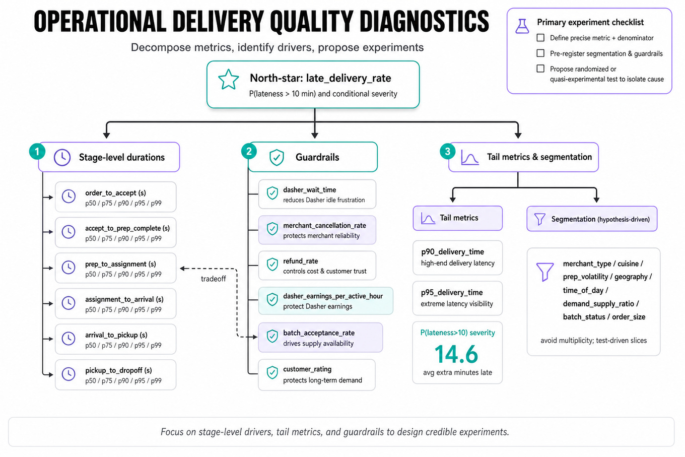
DoorDash is probing whether you can turn an operational symptom like cold food, late deliveries, or Dasher wait time into a rigorous diagnostic analytics and experimentation plan. A strong Data Scientist should define the right metric, decompose the end-to-end delivery funnel, isolate likely causes using observational data, and propose credible tests that distinguish correlation from causation. DoorDash cares because small changes in prep time, dispatch timing, routing, batching, or merchant handoff can materially affect customer retention, Dasher earnings, merchant trust, and marketplace efficiency. The interviewer is looking for structured thinking, statistical judgment, and an ability to balance marketplace tradeoffs rather than jumping to one explanation.

Core knowledge

• End-to-end order lifecycle decomposition is the backbone: order created → merchant accepts → food prep → Dasher assigned → Dasher arrives at merchant → pickup → travel to customer → dropoff. Most delivery-quality metrics should be decomposed into stage-level durations before proposing interventions.

• Primary metrics should map directly to customer harm, e.g. late_delivery_rate, cold_food_complaint_rate, avg_delivery_lateness, or p90_delivery_time. Use a rate denominator carefully: complaints per delivered order can be biased by customer propensity to complain, while app-observed lateness is broader but less directly tied to sentiment.

• Guardrail metrics prevent local optimization. For late deliveries, guardrails might include dasher_wait_time, merchant_cancellation_rate, refund_rate, dasher_earnings_per_active_hour, batch_acceptance_rate, and customer_rating. Reducing lateness by over-dispatching Dashers may improve customer ETAs while harming Dasher utilization.

• Metric decomposition should separate mean effects from tail effects. DoorDash quality issues often live in the right tail, so track p50, p75, p90, p95, and p99, not just averages. For lateness, define $lateness = actual\_delivery\_time - quoted\_delivery\_time$ and analyze both $P(lateness > 10)$ and conditional severity.

• Segmentation should be hypothesis-driven: merchant type, cuisine, prep-time volatility, geography, market density, time of day, weather, order size, distance, batching status, Dasher supply-demand ratio, and new versus repeat customers. Avoid slicing into hundreds of cohorts without multiplicity control or a prior rationale.

• Counterfactual thinking matters because marketplace metrics are confounded. Rain can increase both delivery times and complaint rates; busy merchants may have longer prep times and more complex orders. Use matching, regression adjustment, difference-in-differences, or fixed effects to estimate whether a suspected driver actually caused the spike.

• Difference-in-differences is useful when a change affects some markets, merchants, or time windows but not others. The basic estimand is $(Y_{treated,post}-Y_{treated,pre})-(Y_{control,post}-Y_{control,pre})$. The key assumption is parallel trends, which you should validate visually and with pre-period placebo checks.

• Regression modeling can quantify drivers but should not be oversold as causal. A model like cold_complaint ~ delivery_time + wait_time + distance + weather + cuisine + market_fixed_effects + hour_fixed_effects helps prioritize hypotheses. Interpret coefficients cautiously when features are downstream of each other.

• Experiment design should match the intervention level. If changing dispatch timing, randomize at order or merchant-market-time level depending on interference. If Dashers can receive both treatment and control orders in the same shift, spillovers can contaminate estimates; cluster randomization may be cleaner but lower-powered.

• Power analysis should be discussed for rare events like cold-food complaints. For a binary metric, approximate sample size per arm scales as $n \approx 16p(1-p)/\delta^2$ for 80% power and 5% two-sided alpha under common assumptions. If baseline complaint rate is 2%, detecting a 5% relative lift requires very large samples.

• Instrumentation quality is fair game from an analysis lens: know which signals you would query, such as GPS pings, merchant tablet timestamps, ETA quotes, Dasher arrival events, customer complaint labels, refund reasons, weather, and support tickets. Do not design pipelines; instead, state how you would validate timestamp consistency, missingness, and label bias.

• Marketplace interference is a central edge case. Treating one set of orders can affect Dasher availability, merchant congestion, or batching opportunities for untreated orders. For high-interference interventions, prefer market-level switchbacks, geo experiments, or time-block randomization over naive user-level A/B tests.

Worked example

For Diagnose cold-food spike and design experiments, a strong first 30 seconds would clarify: “Is the spike in complaint rate, refund rate, low ratings mentioning temperature, or all of them? Is it localized by market, merchant, cuisine, weather, or time? Did any product, dispatch, batching, or ETA policy change recently?” I would define the primary metric as cold_food_complaint_rate = cold_food_complaints / delivered_orders, with supporting metrics like delivery_duration_after_pickup, dasher_wait_time, merchant_prep_time, batch_rate, distance, refund_rate, and customer_rating.

The answer should be organized around four pillars: validate the metric, localize the spike, form causal hypotheses, and design interventions. First, I would check whether the complaint-label mix changed, because a support taxonomy or in-app prompt change could create an artificial spike. Second, I would decompose the lifecycle to see whether cold complaints correlate more with long post-pickup travel, long Dasher wait after food is ready, excessive batching, weather, or certain cuisines with low heat retention. Third, I would compare affected versus unaffected cohorts using pre/post trends, merchant fixed effects, weather controls, and distance controls.

A specific tradeoff to flag: reducing cold food by assigning Dashers earlier may reduce post-ready wait, but it can increase dasher_wait_time at merchants and lower Dasher earnings per active hour. For experiments, I might test a revised dispatch rule for high-risk orders, such as hot-food cuisines during cold weather and long-distance trips, randomizing at merchant-market-time blocks to reduce interference. The primary success metric would be cold complaints, while guardrails include late delivery, Dasher wait, cancellation, batching efficiency, and customer reorder rate. I would close by saying that, with more time, I would build a risk model for cold-food probability and evaluate whether targeted interventions outperform blanket dispatch changes.

A second angle

For Investigate Causes of Increased Driver Wait Time, the same diagnostic playbook applies, but the customer-facing symptom is less direct and the unit economics tradeoff is more explicit. I would define dasher_wait_time as time from Dasher arrival at merchant to pickup, then segment by merchant, cuisine, order size, prep-time estimate accuracy, acceptance time, and peak-hour congestion. The causal hypotheses shift toward merchant prep delays, early dispatch, inaccurate ready-time predictions, and pickup process friction. The experiment might test later dispatch or improved prep-time prediction, but guardrails become late_delivery_rate, customer_wait_time, and dasher_utilization. Unlike cold-food complaints, this metric is observed for nearly every order with valid GPS and pickup timestamps, so power is usually easier, but timestamp accuracy and arrival geofence definitions become more important.

Common pitfalls

Pitfall: Jumping straight to “bad weather caused it” without a counterfactual.

Weather is a plausible driver of late or cold deliveries, but it often coincides with demand spikes, Dasher supply shortages, and merchant congestion. A better answer compares similar markets or time windows with and without weather shocks, controls for demand and supply, and checks whether the spike remains after decomposition.

Pitfall: Defining one metric and ignoring marketplace guardrails.

A tempting answer is “optimize delivery time” or “reduce complaints” in isolation. DoorDash problems are multi-sided: an intervention can help customers while hurting Dashers or merchants, so strong candidates explicitly define primary, secondary, and guardrail metrics before proposing experiments.

Pitfall: Over-fragmenting the analysis into endless cuts.

Listing every possible segment sounds thorough but can signal lack of prioritization. Start with the order lifecycle, identify where the metric moved most, then segment within that stage using hypotheses; if many comparisons are run, mention false discovery risk and validation on a holdout period.

Connections

Interviewers may pivot from this topic into A/B testing, causal inference, marketplace experimentation, or ETA model evaluation. Be ready to discuss switchback experiments, interference, power for low-base-rate metrics, and how offline diagnostics translate into online decision-making.

Further reading

• Trustworthy Online Controlled Experiments by Kohavi, Tang, and Xu — practical foundation for experiment design, guardrails, novelty effects, and decision quality.

• Causal Inference: The Mixtape by Scott Cunningham — accessible treatment of difference-in-differences, fixed effects, and causal identification.

• Mostly Harmless Econometrics by Angrist and Pischke — deeper reference for regression, natural experiments, and credible empirical strategy.

Practice questions

What's being tested

DoorDash is probing whether you can design causal experiments in a marketplace where one user’s treatment can affect another user’s outcome. Classic user-level A/B tests often fail because supply, demand, prices, batching, dispatch, and delivery times are coupled within a local market. A strong Data Scientist answer shows that you can choose the right randomization unit, control interference, define marketplace-wide metrics, and analyze results with appropriate fixed effects, clustered uncertainty, and operational guardrails. Interviewers are looking for practical judgment: not “run an A/B test,” but “what experiment is valid for this marketplace mechanism, and what tradeoffs does it create?”

Core knowledge

• Marketplace interference occurs when treatment changes the shared environment: available Dashers, delivery ETAs, restaurant prep queues, batching opportunities, or consumer conversion. If treated users consume scarce supply, control users may see worse ETA, causing a biased estimate of treatment impact.

• SUTVA — the Stable Unit Treatment Value Assumption — is often violated in delivery marketplaces. The assumption says each unit’s outcome depends only on its own treatment. For DoorDash, that can fail because orders, Dashers, merchants, and consumers interact through shared local supply-demand balance.

• Switchback experiments randomize treatment by geography-time cells, such as market_id × hour or zone × daypart, instead of by user. The treatment switches on and off over time within the same market, reducing contamination when marketplace state is shared locally.

• Randomization unit choice should match the interference radius. For dispatch, batching, fees, or delivery promises, prefer zone × time or market × time. For consumer UI copy with minimal supply effects, user-level randomization may be acceptable. For merchant prep changes, merchant-level or geo-level designs may be cleaner.

• Primary metrics should reflect the full marketplace objective, not one side only. Common DoorDash metrics include order_volume, conversion_rate, gross_order_value, contribution_profit, delivery_time, ETA_accuracy, Dasher_utilization, Dasher_earnings, cancellation_rate, refund_rate, and merchant acceptance or prep latency.

• Guardrail metrics catch harms hidden by the primary metric. For example, order batching may improve Dasher_utilization and profit but worsen delivery_time, cold food complaints, NPS, or reorder rate. A fee increase may improve per-order margin but reduce conversion or long-run retention.

• Difference-in-differences with fixed effects is a common analysis frame for switchbacks:
  $Y_{g,t} = \alpha_g + \gamma_t + \beta T_{g,t} + \epsilon_{g,t}$
  where $g$ is geography, $t$ is time, $\alpha_g$ controls persistent market differences, and $\gamma_t$ controls common time shocks.

• Clustered standard errors are usually required because observations within a market-time cell are correlated. If treatment is assigned at zone × hour, uncertainty should be clustered at the randomization level or higher. Treating millions of orders as independent can massively overstate significance.

• Power calculations should use the effective sample size of randomized cells, not raw orders. A test with 50 markets over 14 days and 4 dayparts has roughly $50 × 14 × 4 = 2{,}800$ assignment cells before accounting for autocorrelation, imbalance, and clustering.

• Stratification and blocking improve precision. Randomize within market, day of week, and daypart so treatment and control both cover lunch, dinner, weekdays, weekends, high-demand zones, and low-demand zones. This is especially important when demand is highly seasonal or weather-sensitive.

• Carryover effects can bias switchbacks if treatment changes future states. For example, a bad delivery experience in a treated period may reduce future orders in a control period, or Dasher positioning from one hour may affect the next hour. Use washout periods or coarser time blocks when carryover is plausible.

• Noncompliance and partial exposure should be measured explicitly. If a batching algorithm is “on” but only affects 20% of eligible orders, analyze both intent-to-treat and exposure-adjusted effects carefully. ITT preserves randomization; treatment-on-treated estimates need stronger assumptions.

Worked example

For Design and analyze a switchback experiment, a strong candidate would start by clarifying the intervention, the marketplace surface it affects, and the interference radius: “Is this changing dispatch, pricing, batching, or consumer experience, and does it affect shared Dasher supply within a zone?” They would state that a user-level A/B test is likely invalid if the treatment changes supply allocation or delivery timing, because treated and control orders compete for the same Dashers.

The answer should be organized around four pillars: randomization design, metric framework, statistical analysis, and operational risks. For design, propose randomizing zone × time block, such as zone-by-2-hour windows, stratified by market, day of week, and daypart. For metrics, define a primary marketplace metric like contribution_profit_per_order or orders_per_consumer_session, plus guardrails such as delivery_time, cancellation_rate, Dasher_earnings, and merchant_lateness.

For analysis, aggregate outcomes to the assignment cell and estimate a regression with zone fixed effects and time fixed effects, using standard errors clustered by zone or assignment cell. A specific tradeoff to flag is time-block length: shorter blocks create more randomized units and power, but increase carryover risk because Dasher locations and batching queues persist across adjacent periods. Longer blocks reduce carryover but create fewer independent observations and may be more exposed to demand shocks.

A strong close would say: “If I had more time, I’d run pre-experiment simulations using historical order streams to estimate power, check balance, select block length, and stress-test sensitivity to clustering and carryover.”

A second angle

For Evaluate Impact of $1 Fee on Fast-Food Profitability, the same interference logic applies, but the treatment is a pricing change rather than an operational algorithm. A naive consumer-level A/B test may appear reasonable, but if the fee reduces demand in some areas, it can free Dasher supply, improve ETAs, and indirectly affect control consumers nearby. The randomization unit could be consumer-level if the fee is small and supply effects are negligible, but market-time randomization is safer if demand shifts are expected to alter delivery speed or Dasher allocation.

The metric frame also changes: the primary metric should be something like profit_per_visitor or contribution_profit_per_session, not just fee revenue per order. The candidate should explicitly decompose impact into conversion loss, order mix changes, average basket size, delivery cost, refund/cancel rates, and repeat behavior.

Common pitfalls

Pitfall: Saying “randomize users 50/50 and compare average order value” for dispatch, batching, or supply-sensitive changes.

That answer ignores interference. A better response explains why treated and control users share Dashers and restaurants, then proposes geo-time randomization or a switchback design that aligns assignment with the level where marketplace state is shared.

Pitfall: Optimizing one side of the marketplace while ignoring the others.

For example, adding bicycle Dashers might improve supply density and reduce cost in dense zones, but could worsen long-distance delivery times, Dasher earnings mix, or merchant pickup congestion. Strong answers define consumer, Dasher, merchant, and business metrics, then name the intended primary metric and guardrails.

Pitfall: Treating order-level rows as independent observations.

If 200,000 orders come from 500 randomized zone-hour cells, the experiment has closer to hundreds of independent units than hundreds of thousands. The right move is to analyze at the assignment-cell level or use fixed effects with clustered standard errors, then discuss power in terms of clusters and intraclass correlation.

Connections

Interviewers may pivot from this topic into causal inference, especially difference-in-differences, synthetic controls, CUPED, and heterogeneous treatment effects. They may also ask about marketplace metric design, pricing experimentation, ranking and dispatch evaluation, or diagnosing a launch where conversion_rate, ETA, and profit move in opposite directions.

Further reading

• Kohavi, Tang, and Xu, Trustworthy Online Controlled Experiments — Practical treatment of online experiments, guardrails, variance reduction, and common validity threats.

• Blake and Coey, “Why Marketplace Experimentation Is Harder Than It Seems” — Seminal discussion of interference and marketplace experiment design, especially for two-sided platforms.

• Angrist and Pischke, Mostly Harmless Econometrics — Strong foundation for fixed effects, clustered standard errors, difference-in-differences, and causal interpretation.

Practice questions

What's being tested

DoorDash is probing whether a Data Scientist can evaluate pricing, incentive, and fulfillment changes through the lens of unit economics, causal inference, and marketplace experimentation. Strong answers connect customer behavior, merchant pricing, Dasher supply, and contribution margin without drifting into engineering or purely strategic hand-waving. Interviewers are looking for metric judgment: what is the right success metric, what are the guardrails, how would you estimate impact credibly, and how would you handle interference across a three-sided marketplace? The best candidates can reason from both experimental evidence and observational data, quantify uncertainty, and explain tradeoffs between growth, profitability, and marketplace health.

Core knowledge

• Unit economics means measuring profit per transaction, user, merchant, geography, or cohort. A basic delivery-order margin frame is:
  $\text{Contribution Profit} = \text{Consumer Fees} + \text{Commission} + \text{Ad Revenue} - \text{Dasher Pay} - \text{Promos} - \text{Refunds/Credits} - \text{Payment/Support Costs}.$
  Clarify whether fixed costs are excluded.

• Pricing changes affect both revenue and demand, so never evaluate a fee only by incremental dollars per order. Estimate $\Delta \text{Profit} = \Delta \text{Revenue} - \Delta \text{Variable Cost}$ while accounting for changes in conversion_rate, order_frequency, AOV, retention, refund_rate, and Dasher_utilization.

• Elasticity is central for fee and menu-price questions. Own-price elasticity is often approximated as:
  $E = \frac{\%\Delta Q}{\%\Delta P}.$
  If a $1 fee raises order price by 5$-0.6$. Segment by cuisine, income proxy, geography, new versus existing users, and time of day.

• Marketplace interference is a major experimental risk. Treating consumers may change Dasher availability, delivery times, merchant batching, or marketplace liquidity for control users. For strong interference, prefer geo-randomization, switchback experiments, market-level randomization, or cluster-robust inference over naive user-level A/B testing.

• Randomization unit should match the mechanism. A consumer fee can often randomize by user, but Dasher programs or fulfillment modes may require randomizing by market, zone, or time block. Merchant price inflation analyses are usually observational, requiring matched item panels and careful sampling rather than simple randomized experiments.

• Primary metrics should reflect the business decision. For a fee test, the likely primary metric is contribution_profit_per_visitor or contribution_profit_per_order, not just revenue_per_order. Guardrails include order_volume, conversion_rate, delivery_time, refund_rate, merchant_cancellations, Dasher_acceptance_rate, and customer retention.

• Intent-to-treat estimates are usually the default for experiments: compare all users assigned to treatment versus control, regardless of exposure. If only some users see the fee, report both ITT and treatment-on-treated using exposure or instrumental-variable logic, but do not let post-treatment filtering bias the result.

• Sample size and power matter because profit metrics are noisy. For a two-sample mean comparison, a rough per-arm sample size is:
  $n \approx \frac{2\sigma^2(z_{1-\alpha/2}+z_{1-\beta})^2}{\delta^2}.$
  Use historical variance for profit_per_user, not just order-level variance, and account for clustering if randomizing by market.

• Heterogeneous treatment effects are often the story in pricing. A fee may improve profit in dense urban markets but reduce conversion in suburban areas; bike couriers may reduce cost downtown but hurt ETA in low-density zones. Pre-specify key cuts to avoid cherry-picking: geography, customer tenure, merchant vertical, basket size, and supply-demand balance.

• Observational price inflation studies need matched merchant-item panels. Compare DoorDash menu prices versus in-store prices for the same item, merchant, geography, and time period. Watch for item substitutions, menu reclassification, taxes/fees excluded from menu price, and survivorship bias if discontinued items vanish from the panel.

• Forecasting inflation gaps should separate signal from sampling noise. Use weighted averages by order volume or merchant mix, report confidence intervals via bootstrap or cluster-robust standard errors, and consider simple baselines before complex models: seasonal naive, ARIMA, exponential smoothing, or hierarchical time-series models by category and market.

• Decision quality requires translating estimates into launch logic. A statistically significant lift in revenue_per_order may still be a bad launch if long-term retention falls or if Dasher supply worsens. Conversely, a small average effect may be compelling if concentrated in large, profitable segments with clean guardrails.

Worked example

For **“Evaluate Impact of $1 Fee on Fast-Food Profitability,”** start by clarifying whether the$1 applies to all fast-food orders, a subset of users, specific markets, or certain basket sizes, and whether the goal is short-term contribution profit or long-term customer value. In the first 30 seconds, state that you would evaluate both incremental margin and demand response, because the fee mechanically increases revenue per completed order but may reduce conversion or frequency. Organize the answer around four pillars: experiment design, metric framework, interference/segmentation, and decision criteria.

For design, propose a randomized experiment at the consumer or market level depending on expected spillovers; if fast-food demand affects local Dasher availability, geo or zone-level randomization is safer. For metrics, use contribution_profit_per_eligible_user as the primary metric, with secondary diagnostics like orders_per_user, conversion_rate, AOV, fee_revenue, Dasher_pay_per_order, and refund_rate. For guardrails, include delivery_time, customer_retention, merchant_cancellations, and customer support contacts. Explicitly flag the tradeoff between user-level randomization, which is more powered, and market-level randomization, which better protects against marketplace interference. Close by saying that, with more time, you would estimate heterogeneous effects by market density, basket size, customer tenure, and competitor sensitivity before recommending a broad launch or targeted rollout.

A second angle

For “Assess Success Criteria for Bike-Courier Delivery Launch,” the same unit-economics logic applies, but the intervention changes fulfillment cost and reliability rather than consumer price. The primary question becomes whether bike couriers improve contribution_profit_per_order by lowering Dasher pay, parking delays, or batching inefficiency without worsening ETA, cancellation, or courier supply health. Randomization may need to happen by zone and time window because delivery supply is shared, making user-level treatment less credible. The analysis should also segment by density, distance, weather, order size, and merchant type because bikes may work well for short downtown trips but fail for long suburban routes. Instead of elasticity, the key mechanism is operational cost-to-serve and service quality impact.

Common pitfalls

Pitfall: Treating revenue lift as profit lift.

A tempting answer is “a $1 fee increases revenue by$1 per order, so profitability improves.” That ignores fewer orders, different basket composition, higher refunds, retention effects, and potential Dasher or merchant cost changes. A stronger answer anchors on contribution_profit_per_eligible_user and decomposes the result into price, volume, and cost components.

Pitfall: Ignoring marketplace interference.

A naive A/B test can look clean statistically while violating the stable unit treatment value assumption. If treated customers reduce demand, control customers may see faster delivery or better Dasher availability, contaminating the estimate. Call out interference early and justify the randomization unit rather than defaulting to user-level assignment.

Pitfall: Overfitting the narrative with too many segments.

Segmentation is valuable, but listing twenty cuts without a plan sounds like fishing. Pre-specify the few segments tied to mechanism: density for bike couriers, basket size for fees, cuisine or merchant type for price inflation, and tenure for retention sensitivity. Then use exploratory cuts only to generate follow-up hypotheses.

Connections

Interviewers may pivot from here into experimental design, especially cluster randomization, switchbacks, power analysis, and sequential monitoring. They may also ask about causal inference for non-randomized launches, time-series forecasting for inflation gaps, or metric design for marketplace health and profitability.

Further reading

• Trustworthy Online Controlled Experiments — Kohavi, Tang, and Xu’s practical guide to experiment design, metrics, guardrails, and pitfalls.

• Causal Inference: The Mixtape — accessible treatment of difference-in-differences, matching, instrumental variables, and causal identification.

• Mostly Harmless Econometrics — rigorous foundation for applied causal inference in observational business settings.

Practice questions

Statistics & Math

What's being tested

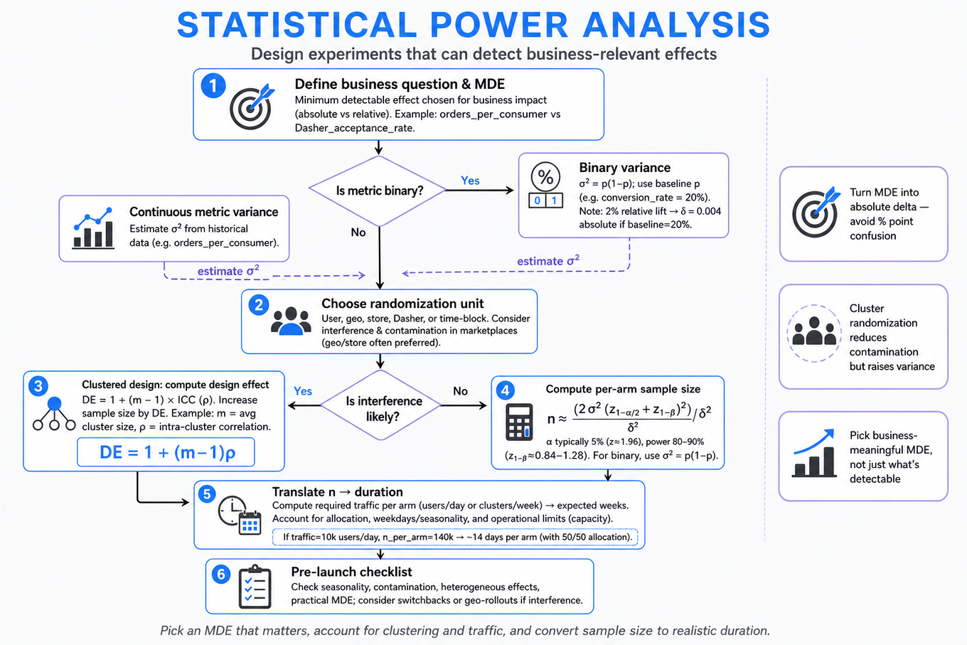
Statistical power analysis in these interviews is about whether you can design an experiment that has a realistic chance of detecting a business-relevant effect before DoorDash spends weeks running it. The interviewer is probing whether you understand the link between effect size, variance, sample size, randomization unit, and experiment duration, especially in marketplace settings with interference between consumers, Dashers, and merchants. You are expected to reason beyond a simple user-level A/B test: switchbacks, geo launches, notification campaigns, courier initiatives, and revenue algorithms all create clustering, contamination, seasonality, and heterogeneous treatment effects. DoorDash cares because underpowered tests waste marketplace capacity, while overpowered or poorly framed tests can ship statistically significant but operationally meaningless changes.

Core knowledge

• Power is the probability of detecting a true effect of a specified size: $1 - \beta$, commonly set to 80% or 90%. The standard test design also chooses a Type I error rate $\alpha$, often 5%, and a practically meaningful minimum detectable effect.

• MDE should come from product or business relevance, not from whatever the experiment can conveniently detect. For DoorDash, a 0.1% lift in orders_per_consumer may matter at scale, while a 0.1% lift in Dasher_acceptance_rate may be meaningless if it worsens on_time_delivery_rate.

• For a two-sample difference in means with equal allocation, approximate per-arm sample size is:
  $n \approx \frac{2\sigma^2(z_{1-\alpha/2}+z_{1-\beta})^2}{\delta^2}$
  where $\sigma^2$ is outcome variance and $\delta$ is the absolute MDE. Binary metrics use $\sigma^2=p(1-p)$.

• Relative MDE and absolute MDE must be translated carefully. If baseline conversion_rate is 20%, a 2% relative lift means $\delta=0.004$ absolute, not 0.02. Many weak interview answers overstate power by confusing percentage points with percent lift.

• Randomization unit determines effective sample size. User-level randomization works for independent consumer experiences, but marketplace experiments often need cluster randomization by geo, store, Dasher, or time block to reduce interference. More rows in the dataset do not imply more independent observations.

• Clustered designs inflate variance through the intra-cluster correlation. A common design effect is:
  $DE = 1 + (m-1)\rho$
  where $m$ is average cluster size and $\rho$ is the intra-cluster correlation. Effective sample size is roughly $n_\text{raw}/DE$, which can drastically reduce power for geo or store-level tests.

• Switchback experiments randomize treatment by market-time blocks, such as city-hour or zone-day. Power depends on the number of randomized blocks, not just total orders. Analysis should usually include fixed effects for market and time, plus clustered standard errors at the randomization level.

• Pre-period covariates can improve power through CUPED or regression adjustment. If a covariate $X$ explains outcome variance, adjusted variance becomes approximately $\sigma_Y^2(1-\rho_{YX}^2)$. This is valuable for noisy metrics like gross_order_value, delivery_time, and retention.

• Triggering affects power and interpretation. If only 10% of consumers receive an extra notification, analyzing all assigned users estimates the intent-to-treat effect and may be diluted. A triggered analysis can improve sensitivity but risks post-treatment selection bias unless eligibility is defined pre-randomization.

• Ratio metrics such as revenue_per_order, orders_per_active_user, or cost_per_delivery need careful variance estimation. Delta method, bootstrap, or user-level aggregation is often safer than treating numerator and denominator events as independent.

• Multiple metrics create multiple testing risk. DoorDash experiments usually have one primary metric, guardrails such as refund_rate, lateness, and Dasher_pay, and diagnostic secondary metrics. Use hierarchy, pre-registration, or corrections like Bonferroni or Benjamini-Hochberg when many claims are made.

• Duration must cover temporal cycles. Even if sample size is reached in two days, marketplace metrics often vary by weekday, lunch/dinner peaks, weather, holidays, and promotions. A credible design often runs at least one or two full weekly cycles unless the intervention is extremely short-lived.

Worked example

For Design and analyze a switchback experiment, a strong candidate would start by clarifying the intervention, the marketplace side affected, the primary metric, and the likely interference pattern: “Are we changing dispatch logic, pricing, batching, or Dasher incentives, and does treatment spill over across nearby zones or time windows?” They would state that user-level randomization may be invalid if supply is shared, so they would propose randomizing market-time blocks, such as zone_id × hour or market × meal_period. The answer would be organized around four pillars: define success metrics and guardrails, choose the randomization unit, calculate power/MDE using block-level variance, and specify the analysis model.

For the model, they might propose a regression like $Y_{zt}=\alpha_z+\gamma_t+\tau T_{zt}+\epsilon_{zt}$, where $\alpha_z$ are zone fixed effects, $\gamma_t$ are time fixed effects, and standard errors are clustered by zone or switchback block depending on assignment. They would explain that power comes from the number of randomized blocks and the within-zone over-time variation, not merely the number of deliveries. A key tradeoff is granularity: shorter blocks increase sample size but raise carryover risk if Dashers reposition or orders started in one block finish in another. They would close by saying that, with more time, they would simulate power from historical delivery_time, fulfillment_rate, and order_volume data to account for skew, seasonality, and cluster correlation instead of relying only on a normal approximation.

A second angle

For Analyze Retention Data for Geo-Targeted Feature Launch, the same power logic applies, but the constraint shifts from time-block randomization to a small number of geographies. The effective sample size is closer to the number of markets than the number of consumers, especially if local marketing, merchant mix, or Dasher supply shocks affect everyone in a region. A strong design would use matched geo pairs, pre-period retention trends, and possibly a difference-in-differences estimator to reduce variance. Power should be based on historical market-level retention volatility, not individual-level binomial variance. The candidate should also discuss that retention curves create multiple endpoints, such as D7_retention, D28_retention, and repeat-order rate, so the primary endpoint must be chosen before launch.

Common pitfalls

Pitfall: Treating rows as independent observations.

A tempting answer is, “We have millions of orders, so the experiment will be highly powered.” That fails in switchback, geo, courier, and marketplace tests because the independent unit may be a zone-hour, market, Dasher, or user cohort. A better answer explicitly identifies the randomization unit and computes power using variance at that level.

Pitfall: Starting with the formula before defining the decision.

Interviewers do not want a memorized sample-size equation detached from the business question. If the candidate cannot say what MDE matters for revenue, retention, delivery_quality, or Dasher_experience, the math is not useful. Start with the decision the experiment must support, then translate that into an effect size and duration.

Pitfall: Ignoring dilution and noncompliance.

For notification experiments or courier initiatives, not everyone assigned to treatment will actually receive or comply with the treatment. Reporting only a per-exposed lift can exaggerate impact if exposure is post-treatment. A stronger answer distinguishes intent-to-treat, treatment-on-the-treated, eligibility criteria, and how each affects power and causal interpretation.

Connections

Interviewers often pivot from power analysis into causal inference, especially difference-in-differences, instrumental variables, or synthetic control for geo launches. They may also probe metric design, experiment guardrails, sequential testing, variance reduction, or heterogeneous treatment effects across markets, merchants, consumers, and Dashers.

Further reading

• Trustworthy Online Controlled Experiments — Kohavi, Tang, and Xu; practical reference for online experimentation, variance, guardrails, and interpretation.

• Field Experiments: Design, Analysis, and Interpretation — Gerber and Green; strong treatment of randomization, clustering, and causal estimands.

• Causal Inference for Statistics, Social, and Biomedical Sciences — Imbens and Rubin; deeper foundation for potential outcomes, assignment mechanisms, and experimental validity.

Practice questions

Machine Learning

What's being tested

DoorDash Data Scientist interviews on this topic test whether you can turn messy marketplace prediction problems into decision-ready models, not just optimize an offline score. You are expected to define the target, prevent temporal leakage, choose evaluation metrics that map to business costs, and explain how model outputs would change dispatch, ranking, promotions, or customer communication. DoorDash cares because ETA accuracy, late-delivery risk, restaurant ranking, courier incentives, and uplift targeting directly affect conversion, on-time delivery, refund rate, Dasher utilization, and marketplace balance. The interviewer is probing for statistical judgment: how you would know the model is valid, whether it is calibrated, whether it causes better outcomes, and what guardrails prevent harm to customers, Dashers, or merchants.

Core knowledge

• Target definition is the first modeling decision. For late-delivery risk, specify “late relative to promised delivery window by > X minutes” rather than vague lateness. For ETA, distinguish actual delivery duration, quoted ETA error, and customer-perceived lateness; each leads to different labels and interventions.

• Temporal validation is mandatory in delivery prediction. Train on weeks 1–6, validate on week 7, test on week 8, preserving event time. Random splits leak future restaurant behavior, Dasher supply patterns, weather, batching logic, and marketplace conditions into the training distribution.

• Feature leakage often appears as “helpful” operational signals. Post-assignment pickup time, actual Dasher arrival, customer support contact, cancellation reason, or final route duration cannot be used for pre-dispatch prediction. A strong answer states feature availability at decision time: checkout, assignment, pickup, or en route.

• Model class choice should match interpretability, nonlinearity, and actionability. Logistic regression gives calibrated, explainable baselines; XGBoost or LightGBM often perform well on tabular marketplace data with nonlinear interactions; quantile regression or gradient-boosted quantiles are useful for ETA uncertainty.

• Calibration matters when predictions drive thresholds. A model with AUC = 0.85 can still overstate risk. Use reliability plots, calibration-in-the-large, expected calibration error, and bin-level checks: for orders scored 0.20 risk, about 20% should be late. Consider isotonic regression or Platt scaling.

• Ranking metrics depend on whether the model is used for ordering or absolute decisions. Use NDCG@K, MAP, pairwise accuracy, or top-decile lift for ranking; use AUC, PR-AUC, log loss, and calibration for probability decisions. For rare events, PR-AUC is often more informative than AUC.

• Cost-sensitive decisioning converts predictions into actions. If intervention cost is $c$ and expected late-delivery loss is $L$, intervene when $p(\text{late}) \times L > c$. With capacity constraints, sort by expected incremental value, not raw risk, because high-risk orders may not be fixable.

• Uplift modeling estimates treatment effect heterogeneity: $\tau(x)=E[Y(1)-Y(0)\mid X=x].$ For promotions, incentives, or proactive support, ranking by predicted outcome risk is not enough; prioritize users or orders with high incremental response. Evaluate using Qini curves, uplift@K, and randomized holdouts.

• ETA modeling is both point prediction and uncertainty estimation. Optimize MAE or pinball loss for robust estimates, but also evaluate coverage: a predicted 80% interval should contain the actual delivery time about 80% of the time. Underpredicting ETA may increase conversion but harm trust.

• Offline-to-online gaps are common in marketplace ML. A ranking model may improve offline relevance but reduce merchant diversity, increase delivery distance, or overload popular stores. A DS should propose an A/B test with primary metrics, guardrails, segment cuts, and pre-specified launch criteria.

• Segmentation analysis protects against averaged-out failures. Check performance by geography, time of day, cuisine, merchant prep-time volatility, weather, new vs. repeat customers, bike vs. car courier, and order size. A model that helps suburban car deliveries may hurt dense urban bike deliveries.

• Monitoring from a DS lens means watching model quality and business outcomes, not designing pipelines. Track score distribution shifts, calibration drift, feature missingness rates, MAE, late rate, cancellation rate, refund rate, Dasher wait time, and merchant throttling by segment after launch.

Worked example

For Build a late-delivery risk model, a strong candidate would start by clarifying the decision point: “Are we scoring at checkout, Dasher assignment, pickup, or while en route?” They would define the label precisely, such as an order being more than 10 minutes later than the promised ETA, and ask what action the score enables: dispatch adjustment, customer notification, refund prevention, or merchant intervention. The answer should then be organized around four pillars: target and data construction, feature design with availability constraints, validation and evaluation, and decision policy plus monitoring.

For features, they might include merchant historical prep-time variance, current demand-supply ratio in the zone, quoted distance, time of day, weather indicators, basket size, batching status if known at scoring time, and Dasher proximity if scoring after assignment. For validation, they should recommend a rolling time-based split and compare a simple baseline, such as historical late rate by merchant-zone-hour, against logistic regression and LightGBM. Evaluation should include PR-AUC if lateness is rare, calibration curves because scores drive actions, and business-weighted metrics such as expected preventable late minutes or cost per avoided late order.

One explicit tradeoff to flag is recall versus intervention cost: aggressively flagging orders may reduce late deliveries but overuse incentives, customer credits, or manual ops actions. A strong close would say: “If I had more time, I’d estimate which late orders are actually preventable, because a risk model alone may target unavoidable failures; I’d also evaluate fairness across neighborhoods, merchants, and courier modes.”

A second angle

For Evaluate a new ranking model, the same predictive-modeling discipline applies, but the unit of decision is an ordered list of stores or items rather than a single binary risk score. Offline metrics like NDCG@K or predicted conversion lift are useful, but DoorDash needs an experiment because ranking changes customer choice, merchant exposure, delivery distance, and kitchen congestion. The DS framing should include primary metrics such as conversion_rate or order_rate, guardrails like delivery time, cancellation rate, merchant concentration, and Dasher utilization, plus segment analysis for new users, dense markets, and cuisine categories. Unlike late-risk prediction, calibration may be less central than counterfactual bias: historical clicks reflect the old ranking policy, so logged position, impressions, and randomized exploration matter for credible evaluation.

Common pitfalls

Pitfall: Treating predictive accuracy as the business objective.

A tempting answer is “maximize AUC and launch if it improves.” That misses whether predictions are calibrated, actionable, and economically valuable. A better answer translates model scores into decisions, defines intervention thresholds, and evaluates incremental impact through experiments or randomized holdouts.

Pitfall: Ignoring time and decision-point leakage.

Many candidates list features like actual pickup time, final route duration, or support contacts because they correlate strongly with lateness. The interviewer wants you to say when the prediction is made and exclude signals unavailable at that moment. This is especially important in delivery systems where events unfold sequentially.

Pitfall: Giving an ML catalog instead of a marketplace answer.

Saying “I would try random forest, neural nets, and gradient boosting” is shallow unless tied to ETA, ranking, uplift, or dispatch decisions. Stronger communication names the baseline, explains why a model class fits the data, chooses metrics aligned to the action, and calls out marketplace side effects like merchant overload or Dasher wait time.

Connections

The interviewer may pivot from predictive modeling into experimentation, especially how to validate a model-driven policy online. They may also probe causal inference, uplift modeling, ranking evaluation, metric design, or calibration. For marketplace problems, expect follow-ups on heterogeneous effects, guardrail metrics, and why offline model gains may not translate into customer or Dasher outcomes.

Further reading

• The Elements of Statistical Learning by Hastie, Tibshirani, and Friedman — strong foundation for supervised learning, regularization, tree ensembles, and model evaluation.

• Causal Inference for the Brave and True by Matheus Facure — practical treatment of uplift, treatment effects, and causal evaluation for business decisions.

• “Hidden Technical Debt in Machine Learning Systems” by Sculley et al. — useful framing for why model quality must be evaluated alongside monitoring, feedback loops, and system-level effects.

Practice questions