Hudson River Trading Software Engineer Interview Prep Guide

You're weakest on coding algorithms at 2/5 with no solved questions logged, so this plan concentrates on stateful simulations, hash/canonicalization, strings, arrays/grids, and API-style data structure design before Monday. You're comparatively stronger on behavioral leadership at 4/5 and mid-level on system design/software fundamentals, so those stay as quick review rather than a separate deep-dive. For Hudson River Trading, the highlighted angles are low-latency C++/memory behavior, concurrency/networking for real-time systems, robust trading metrics, rolling market-data aggregation, and probability/expected value. With less than one week, budget about 80–85 focused minutes for this cheat sheet, then spend remaining time on timed implementation practice.

Technical Screen — 83 min

Coding & Algorithms

Focus area — Coding self-rating is 2/5 with no solved questions; HRT screens often frame event-ordering as queues, market data, or reactor simulations.

What's being tested

These problems test stateful simulation and precise event ordering: you must model system state over time and produce correct outcomes as events (arrivals, completions, turns) interleave. Interviewers probe ability to convert rules into deterministic update steps, choose the right event structure, and reason about tie-breaking and time advancement.

Patterns & templates

• Event loop simulation — collect events, advance a simulation clock, process next event; common implementation: priority queue via heapq, O(m log m) for m events.

• Greedy single-server queue — track server availability time t_free; for each arrival, start = max(arrival, t_free); update t_free = start + duration.

• Sort-by-time then stable-tie-break — sort(events, key=(time, tie_key)) ensures deterministic handling of simultaneous events.

• Turn-based alternation — maintain an index or boolean flag to toggle collector/player; perform O(1) updates per turn until list exhausted.

• In-place state updates — mutate accumulators (e.g., queue length, collected count) rather than rebuilding structures; saves memory to O(1) beyond input.

• Use integers/64-bit for time — sum of durations can overflow 32-bit; prefer long/int64.

• Batch-processing vs per-event — when arrivals sorted, process contiguous arrivals before advancing completion to reduce heap operations, improving from O(m log m) to near O(m) in practice.

Common pitfalls

Pitfall: Treating simultaneous arrival and completion in arbitrary order — always define and implement a consistent tie-break (e.g., completions before arrivals or vice versa) and state it to the interviewer.

Pitfall: Forgetting server idle time — using only durations without max(arrival, t_free) yields negative waits and wrong completion times.

Pitfall: Using 32-bit integers for accumulated time — large sums cause overflow; use 64-bit types.

Practice these

The practice cards below cover the canonical variants — solve all of them and time yourself.

Practice questions

Focus area — You viewed several coding items but solved none; canonical hash counting is a common fast path for string/array screen problems.

What's being tested

These problems test hash-based counting and canonicalization: converting items to a normalized key and aggregating counts efficiently to answer pair/prefix queries. Interviewers probe correctness (edge cases), time/space complexity, and careful key design to avoid collisions or double-counting.

Patterns & templates

• Frequency map using a hashmap — count canonical keys in O(n) time and O(u) extra space, where u is unique canonical forms.

• Canonical key by transform — apply a deterministic transform (sorted digits, reversal-normalized string, trimmed prefix) before hashing to group equivalents.

• Use combination formula for pairs: for count k, number of unordered pairs is k*(k-1)/2 — avoid nested loops.

• Represent numeric canonical keys as strings when leading zeros matter; otherwise use integer tuples for compactness and faster hashing.

• Streaming accumulation: update counts on the fly, emit pairs incrementally with current count to save memory when needed.

• For prefix problems, build a prefix-hash map or use a trie when many shared prefixes reduce key space; O(L*n) where L is average length.

Common pitfalls

Pitfall: Forgetting leading zeros — treating reversed digits as integers collapses distinct forms like "010" and "10".

Pitfall: Miscounting pairs by summing k instead of using k*(k-1)/2, producing linear instead of combinatorial results.

Pitfall: Creating heavy keys (e.g., full sorted strings) for very long items when a fixed-length hash or tuple would suffice, increasing memory and hash time.

Practice these

the practice cards below cover the canonical variants — solve all of them and time yourself

Practice questions

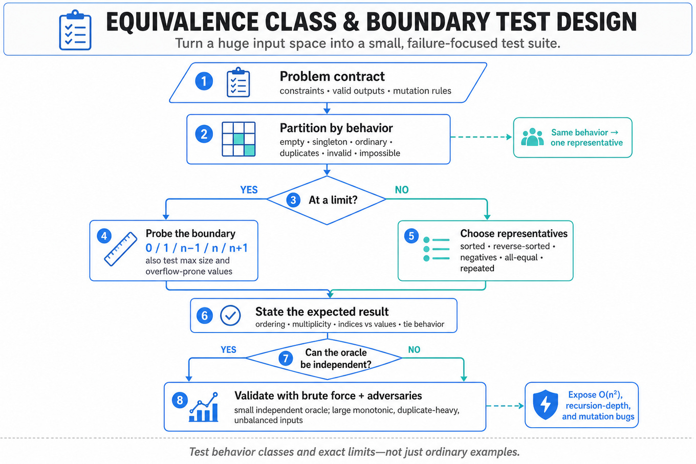
Focus area — Low coding rating and Monday timeline make test design high leverage for avoiding edge-case misses under time pressure.

What's being tested

These questions test equivalence-class partitioning and boundary-value analysis for algorithm and data-structure problems. You must reduce a huge input space into representative valid, invalid, empty, minimal, maximal, duplicate, and adversarial cases, then state precise expected outputs. Strong answers connect each case to a likely implementation failure rather than listing random examples.

Patterns & templates

• Equivalence classes — partition inputs by behavior: empty, singleton, ordinary, duplicate-heavy, invalid, already processed, and impossible-result cases.

• Boundary testing — check values at, just below, and just above limits: 0, 1, n, n-1, maximum size, and overflow-prone magnitudes.

• Array templates — include empty arrays, one element, sorted and reverse-sorted inputs, all-equal values, negatives, repeated values, and answers at both endpoints.

• String templates — test empty strings, one character, whitespace, mixed case, punctuation, repeated characters, Unicode assumptions, and prefixes that almost match.

• Expected outputs — verify ordering, multiplicity, indices versus values, stable tie behavior, and whether the function mutates its input.

• Complexity-aware adversaries — use large monotonic, duplicate-heavy, or highly unbalanced inputs to expose accidental O(n²) behavior or recursion-depth failures.

• Oracle design — derive expected results independently, preferably with a simple brute-force implementation for small inputs; avoid duplicating the candidate algorithm.

Common pitfalls

Pitfall: Testing only ordinary examples misses empty inputs, singleton behavior, duplicate handling, and “no solution” semantics.

Pitfall: Saying “test large inputs” without specifying the exact constraint boundary fails to distinguish n = limit from n = limit + 1.

Pitfall: Confusing invalid-input behavior with a valid empty result; explicitly state whether the API returns an error, sentinel, exception, or empty collection.

Practice these

The practice cards below cover the canonical variants — solve all of them and time yourself.

Practice questions

Software Engineering Fundamentals

Focus area — You explicitly selected concurrency twice, and HRT values safe high-throughput code under contention.

What's being tested

Interviewers probe your ability to build correct, performant, and maintainable concurrent code: safe access to shared state under contention, choice of synchronization primitives, and reasoning about liveness (deadlock/starvation) and memory visibility. At Hudson River Trading, low-latency and high-throughput constraints make tradeoffs between simple correctness (coarse locks) and scalable designs (sharding, lock-free) particularly important. Expect to justify complexity vs. latency, show familiarity with the memory model, and describe measurable mitigations for contention and cache effects.

Core knowledge

• Mutual exclusion (mutex): a blocking primitive that serializes critical sections. Use std::mutex/pthread_mutex_t; cost per lock is low for uncontended cases but grows with context switches and system calls.

• Read-write locks (RWLock): allow concurrent readers, exclusive writers; useful for read-heavy workloads but can starve writers or increase writer latency under high read concurrency.

• Atomic operations and CAS: compare-and-swap (CAS) via std::atomic or __sync_bool_compare_and_swap is the building block for lock-free algorithms; it offers O(1) semantics but may require retry loops under contention.

• Lock-free vs wait-free: lock-free guarantees system progress; wait-free guarantees per-thread progress. Lock-free designs often use CAS loops; wait-free implementations are more complex and rare in production.

• Memory model & happens-before: languages expose ordering (e.g., volatile in Java, memory_order in C++). Correctness depends on establishing happens-before for visibility; otherwise you get data races and undefined behavior.

• Linearizability and correctness criteria: aim for linearizable operations when designing concurrent data structures so each operation appears atomic at some point between invocation and response.

• Liveness hazards: deadlock often stems from inconsistent lock ordering; priority inversion and starvation appear with locks/condition variables and must be mitigated (timeouts, priority inheritance if available).

• Condition variables and spurious wakeups: always use while loops to re-check predicates after wait(); treat wakeups as spurious and re-evaluate state.

• Memory reclamation (ABA problem): lock-free structures need safe reclamation strategies: hazard pointers, epoch-based reclamation, or garbage collection to avoid ABA and use-after-free.

• Contention mitigation patterns: sharding (partition data across locks/cores), per-thread counters with periodic aggregation, exponential backoff in CAS loops, and avoiding false sharing with padding to cache-line boundaries.

Tip: Benchmark with realistic contention patterns (perf, latency p99) and profile cache-misses and lock statistics before over-optimizing.

• False sharing & cache effects: place frequently-updated fields on separate cache lines (align/pad) to prevent ping-ponging and degraded throughput on multi-core systems.

• High-level strategies: prefer simpler locks when contention is low; switch to sharding or lock-free only if profiling shows lock-induced latency or blocking stalls throughput.

Worked example — "Implement a thread-safe LRU cache"

First 30s: clarify capacity, expected read/write ratio, eviction policy ties, required atomicity (single-key atomic vs. global), and persistence/serialization needs. Skeleton answer pillars: (1) data structures: unordered_map for lookup plus doubly-linked list for recency; (2) synchronization: naive global std::mutex for correctness first; (3) performance: sharded cache (N shards each with own map/list and mutex) to reduce contention; (4) eviction: per-shard LRU or global approximate LRU with periodic balancing. Flag tradeoff: a single global lock simplifies correctness and exact LRU but serializes all ops; sharding improves throughput but yields only per-shard LRU (approximate globally). Also mention memory reclamation for nodes if doing lock-free lists. Close by stating further work: measure p99 latency, add metrics (hit-rate, eviction-rate), tune shard count to number of cores, and consider read-mostly optimization with shared_mutex or hazard pointers if lock-free lookup is attempted.

A second angle — "Design a low-contention concurrent counter"

Frame: clarify accuracy (strictly consistent vs. eventual), update rate, and read frequency. Same core concepts apply: atomic increments vs. sharded counters. A basic solution uses std::atomic<uint64_t> for correctness but suffers on multicore under heavy writes. Better: use per-thread or per-core counters (an array indexed by thread-id) and aggregate reads occasionally; this reduces cache bouncing and increases throughput at the cost of slightly stale reads. You'd discuss padding to avoid false sharing and use relaxed memory ordering for increments, while using stronger ordering on aggregation. If exactness is required, combine per-shard counters plus a rare global CAS to reconcile. Emphasize measurement: quantify throughput improvement and staleness tradeoff.

Common pitfalls

Pitfall: assuming atomic++ scales — under high write contention, a single atomic variable becomes a hotspot and kills throughput; prefer sharding or per-thread accumulation.

Pitfall: forgetting spurious wakeups or relying on if around condition_variable::wait() — this yields missed signals and correctness bugs; always re-check the predicate in a loop.

Pitfall: over-promising lock-free correctness without addressing memory reclamation/ABA — a lock-free queue implementation that neglects safe node reclamation will have subtle, crash-prone bugs in production.

Connections

Concurrency interviewers may pivot to adjacent topics like distributed systems consistency (locks → distributed locks, leader election) or performance engineering (profiling, cache behavior, NUMA effects). They might also ask about language-specific models (Java Memory Model, C++ memory_order) or testing strategies for concurrent code (stress tests, fuzzing).

Further reading

• The Art of Multiprocessor Programming — Herlihy & Shavit — canonical book on lock-free/wait-free algorithms and memory models.

• Java Concurrency in Practice — Brian Goetz et al. — practical patterns and pitfalls for concurrency, useful even if not coding in Java.

Practice questions

Focus area — Real-time trading systems depend on message framing, TCP/UDP trade-offs, and failure handling; you also selected distributed resilience topics.

What's being tested

Interviewers are probing your practical fluency with building robust, low-latency networked services: how you pick transports, manage concurrency, reason about latency vs throughput, and design protocols that handle partial failures (retries, timeouts, idempotency). They expect concrete tradeoffs (e.g., blocking threads vs non-blocking I/O) and the right low-level knobs (TCP_NODELAY, buffer sizes, framing) a Software Engineer must use to meet performance and correctness targets.

Core knowledge

• TCP vs UDP semantics: TCP = reliable, ordered, congestion-controlled; UDP = unreliable, unordered, lower latency. Use UDP for multicast/real‑time with application-level recovery.

• Socket API essentials: socket, bind, listen, accept, connect, send, recv, nonblocking EAGAIN behavior; handle partial send/recv and SIGPIPE.

• Non-blocking I/O and readiness APIs: select/poll (O(n) with limits), epoll/kqueue (scales to 10k+ fds), use edge-triggered vs level-triggered semantics deliberately.

• Bandwidth-Delay Product (BDP): BDP = bandwidth * RTT; set send/recv buffers to ~BDP to avoid sender/receiver starvation for high-throughput, high-RTT links.

• Framing strategies: length-prefixed framing versus delimiter-based; use length-prefix + size cap to avoid message-splitting and injection attacks.

• Nagle and delayed ACKs: Nagle's algorithm can increase latency; disable with TCP_NODELAY for small latency-sensitive messages, but consider increased packet count and bandwidth.

• Head-of-line blocking: TCP enforces ordering; multiplexing protocols (e.g., HTTP/2 streams) or UDP-based designs avoid HOL blocking; trade reliability vs complexity.

• Timeouts, retries, idempotency: choose client-side timeouts << overall SLA; implement exponential backoff with jitter; design idempotent RPCs (idempotency keys) so retries are safe.

• TLS cost and session resumption: TLS handshake adds CPU + latency; reuse sessions, enable session tickets, or terminate TLS at trusted endpoints if acceptable.

• Serialization cost: binary formats (protobuf) are more compact and faster to parse than JSON; measure (CPU vs wire savings) before choosing.

• MTU & fragmentation: typical MTU=1500 bytes; avoid UDP fragmentation; enable Path MTU Discovery or send smaller datagrams to avoid reassembly penalties.

• Monitoring & SLOs: track p50, p99, and tail-latency; instrument connect/handshake/send/recv latencies and queue lengths to detect queuing-induced tail spikes.

Worked example

Design a non-blocking TCP server to handle 10k concurrent client connections. First 30 seconds: ask clarifying questions—expected request rate per connection, message size distribution, latency SLOs (p99 target), and whether messages are request/response or streaming. Skeleton answer pillars: (1) use non-blocking I/O with epoll (edge-triggered) and a fixed-size thread pool for processing; (2) implement a small per-connection state machine with length-prefixed framing and a bounded write buffer to handle EAGAIN; (3) apply backpressure so overload drops or rejects new requests early; (4) operational controls: SO_SNDBUF/SO_RCVBUF tuned to BDP, TCP_NODELAY depending on small-message latency need. Tradeoff flagged: edge-triggered epoll requires careful loop to drain sockets or you'll miss events—simpler level-triggered is safer but slightly less efficient. Close: mention metrics to expose (active_connections, send_queue_len, handler_latency), and "if I had more time" you'd add connection pooling, adaptive thread sizing, and stress tests with synthetic traffic to tune buffer sizes.

A second angle

Consider designing a retry and idempotency scheme for RPCs over TLS with strict correctness requirements. The same core concepts apply, but constraints change: TLS increases handshake cost so keep connections pooled and long-lived; retries must consider whether the server processed the request before the connection dropped—use idempotency keys or explicit at-most-once semantics with server-side deduplication. Framing stays length-prefixed, but you must authenticate and authorize each message; add per-RPC unique IDs and persistent logs for dedup checks. Here, latency SLOs push you to choose smaller timeouts and conservative retry counts; additionally, prefer application-level ACKs to know when it’s safe to retry versus assuming retransmission.

Common pitfalls

Pitfall: conflating packet loss with application-level failure.
Many engineers treat a timeout as a permanent failure without distinguishing transient packet loss, server crash, or slow processing; always design retries with increasing backoff and idempotency.

Pitfall: assuming blocking calls are okay at any scale.
Proposing a thread-per-connection model for 10k connections is tempting, but it fails on memory and context-switch costs; explain why event-driven or async I/O scales better.

Pitfall: neglecting framing and partial reads/writes.
Returning a naive recv() loop that assumes one recv() == one message is wrong; always implement buffering and handle partial messages, oversized lengths, and malicious inputs.

Connections

Interviewers may pivot to performance profiling (where to measure CPU vs network stalls) or security (threat model for TLS, certificate rotation, MITM mitigations). They may also ask about distributed-systems reliability patterns like circuit breakers, leader election, or consensus if the protocol needs stronger guarantees.

Further reading

• [TCP/IP Illustrated, Volume 1 — W. Richard Stevens] — classic, deep grounding in TCP/IP behavior and edge cases.

• [High Performance Browser Networking — Ilya Grigorik] — excellent practical coverage of latency, BDP, MTU, and TLS effects on performance.

Practice questions

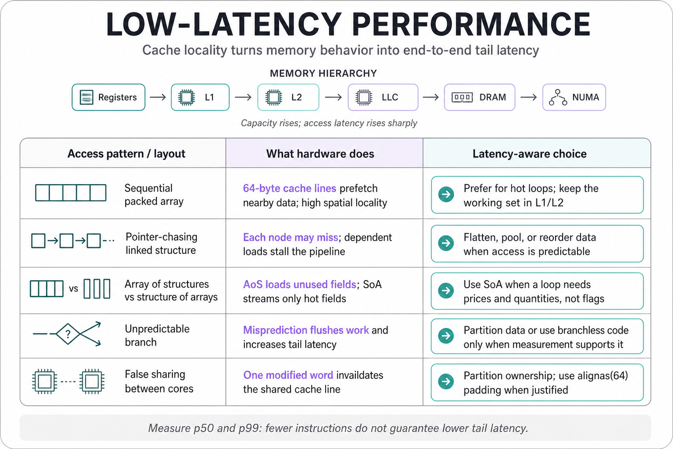
Focus area — HRT-specific addendum: understand cache locality, benchmarking, tail latency, and allocation avoidance for latency-sensitive C++ services.

What's being tested

The interviewer is testing whether you can reason from source code and hardware behavior to end-to-end latency, rather than treating algorithmic complexity as sufficient. You should connect cache locality, memory layout, branch behavior, allocation, synchronization, and measurement to tail latency in a latency-sensitive service. At Hudson River Trading, small and variable delays can affect the timeliness of market-data handling and order decisions, so a strong Software Engineer explains both the optimization and its correctness and maintainability costs.

Core knowledge

• The memory hierarchy has different latency and capacity: registers and L1 are fastest, followed by L2, shared LLC, DRAM, and possibly another NUMA socket. A cache miss can cost tens to hundreds of nanoseconds, vastly more than an arithmetic instruction.

• Spatial locality means nearby addresses are fetched together in a cache line, commonly 64 bytes; temporal locality means recently accessed data is likely to be reused. Sequential iteration over a packed array usually beats pointer-chasing through a linked structure.

• Data-oriented layout often improves locality. An array of structures (struct { price, quantity, flags }) is convenient, but a structure of arrays can avoid loading unused fields when a hot loop needs only prices and quantities.

• Working-set size matters more than nominal input size. Keep hot state within L1/L2 when practical; if a frequently accessed table exceeds cache capacity, reduce the footprint, improve access order, or replace random lookup with a denser representation.

• Cache associativity can create conflict misses even when total data fits in cache. Power-of-two strides, poorly aligned buffers, or several hot arrays mapping to the same sets can cause pathological behavior; padding or changing layout can help.

• False sharing occurs when independent threads modify different words on the same cache line. The line repeatedly invalidates and moves between cores; use ownership partitioning or cache-line padding such as alignas(64) where justified.

• Branch prediction affects both average and tail latency. A predictable branch may be cheap, while an unpredictable branch can stall the pipeline; use data partitioning, branchless operations only when measured beneficial, and avoid assuming branchless code is automatically faster.

• Allocation and indirection add latency and variability. Prefer preallocated storage, object pools, arenas, value types, and contiguous containers on hot paths; account for allocator locks, page faults, destructor work, and garbage-collection pauses where applicable.

• NUMA locality matters on multi-socket machines. A thread accessing memory allocated on another socket can pay additional latency; pin threads, place memory near its owner, and avoid casually sharing mutable state across NUMA nodes.

• Measurement must separate warm and cold behavior. Use representative distributions, warm caches and code paths when measuring steady state, and separately test startup or first-touch behavior. Report median, p99, p99.9, maximum, throughput, and variance rather than only the mean.

• Hardware counters help validate hypotheses. Tools such as `perf` can expose cache references, cache misses, branch misses, cycles, instructions, context switches, and migrations; compare counters before and after a change instead of inferring causality from wall-clock time alone.

• Algorithmic complexity still matters. A cache-friendly $O(n)$ scan can beat an $O(\log n)$ tree for realistic $n$, but an $O(n)$ operation on an unbounded hot path may eventually dominate. State the expected working set, access pattern, and latency budget before choosing.

Worked example

Representative prompt: “How would you optimize a latency-critical order-book data structure?” First, I would clarify the operations, update/read ratio, price-range assumptions, concurrency model, target latency percentile, and whether allocations are allowed on the hot path. I would organize the answer around data representation, access complexity, cache behavior, synchronization, and measurement. For dense bounded price levels, I might use a contiguous price-indexed array for direct lookup; for sparse or unbounded prices, I would compare a sorted array, flat hash table, or tree while considering update costs and locality. I would explicitly flag the tradeoff that a tree offers flexible sparse updates but incurs pointer chasing and poor cache locality, whereas a flat structure may require resizing or more expensive shifts. I would keep ownership with one thread where possible, batch or publish immutable snapshots for readers, and avoid false sharing between per-thread state. I would benchmark replayed production-like update sequences, collect p50 through p99.9, and inspect `perf` counters to confirm whether misses or branches changed. If I had more time, I would test NUMA placement, burst behavior, cancellation-heavy workloads, and correctness under crossed prices and empty levels.

A second angle

Representative prompt: “Why did a seemingly minor code change increase p99 latency?” The framing shifts from selecting a data structure to diagnosing a regression: first compare workload, compiler settings, CPU placement, and measurement methodology. Then inspect changes that enlarge the working set, introduce an allocation, alter alignment, create false sharing, or make a branch less predictable. Averages may remain unchanged while a small fraction of requests suffer cache misses, page faults, preemption, or lock contention, so tail metrics and hardware counters are essential. The best answer proposes a controlled benchmark, a minimal reproducer, and a rollback or targeted change rather than asserting that “cache is slower” without evidence.

Common pitfalls

Pitfall: Analytical mistake — claiming that a contiguous array is always faster or that $O(1)$ lookup guarantees low latency ignores cache capacity, collisions, resizing, branch behavior, and actual access distributions. Explain the workload and validate the claim with measurements.

Pitfall: Communication mistake — listing L1, L2, NUMA, and `perf` terminology without first stating the latency budget, hot operation, and bottleneck makes the answer sound memorized. Start with assumptions and a profiling plan, then connect each optimization to an observed cost.

Pitfall: Depth mistake — recommending padding or lock-free code as a universal fix can increase memory use, complexity, and correctness risk. Discuss ownership, memory ordering, alignment, and whether counters show false sharing or contention before introducing specialized techniques.

Connections

The interviewer may pivot to profiling, benchmark design, lock contention, memory ordering, NUMA, or wait-free and single-producer/single-consumer queues. Be ready to connect locality improvements to algorithmic complexity, concurrency semantics, and tail-latency measurement.

Further reading

• What Every Programmer Should Know About Memory — Ulrich Drepper; detailed treatment of caches, memory hierarchy, NUMA, and locality.

• Computer Architecture: A Quantitative Approach — Hennessy and Patterson; rigorous background on memory systems and performance measurement.

• `perf` Linux manual — practical reference for collecting hardware performance counters and validating optimization hypotheses.

Practice questions

Focus area — Your selected API/OOD, key-value store, and data-structure topics map directly to mutable API invariants and operation complexity.

What's being tested

Candidates must demonstrate designing mutable data-structure APIs that preserve clear invariants while meeting time/space guarantees (often amortized O(1)). Interviewers probe choices for backing representations, how mutation affects indices/state, correctness under concurrent-seeming operations (random sampling, buffered reads), and clear, testable API contracts.

Patterns & templates

• Array + hash map for constant-time membership and removal: store items in an array, map value→index, remove by swapping with last — O(1) amortized.

• Prefix-sum array or alias method for weighted sampling: prefix-sum + binary search O(log n) or alias O(1) for repeated samples; updates cost O(n) vs O(1) with Fenwick tree.

• Circular buffer (ring buffer) for deque semantics with pop_front/push_back in O(1), extend with doubling for amortized O(1) growth.

• Block-deque / unrolled linked list to get O(1) indexable access with segmented arrays, avoiding full-copy shifts.

• Fenwick (BIT) / segment tree to support dynamic weight updates + prefix queries in O(log n) for weighted sampling with updates.

• Internal buffer + cursor for stream-wrapping: persist leftover bytes between calls, return exact requested lengths until EOF; handle mid-call state cleanly.

• Explicit invariants docstring: state what indices mean after each op, exception behavior, and complexity guarantees.

• Test harness templates: randomized ops + oracle (naïve model) to validate correctness under many interleavings.

Common pitfalls

Pitfall: Assuming swapping removal preserves order — it breaks positional semantics; document whether your API preserves order or not.

Pitfall: Using prefix-sum array for weighted sampling without supporting efficient updates — forgets that updates can be O(n) and will timeout at scale.

Pitfall: For stream wrappers, not persisting leftover buffer across calls leads to lost bytes at EOF or incorrect lengths.

Practice these

The practice cards below cover the canonical variants — solve all of them and time yourself.

Practice questions

Focus area — You explicitly selected string parsing/manipulation, and coding rating 2/5 means scan boundaries need extra practice.

What's being tested

These exercises test deterministic string processing: scanning characters or tokens once, maintaining compact state, and enforcing boundary conditions precisely. They probe whether you can translate ambiguous formatting rules into explicit invariants, choose between direct scanning, sorting, and prefix data structures, and state time and space complexity. Hudson River Trading cares because production code often sits on hot paths where predictable O(n) behavior, low allocation, and correct handling of malformed or boundary inputs matter more than clever abstractions.

Core knowledge

• Linear scanning processes each character or token once with a small state machine, giving O(n) time and usually O(1) auxiliary space. Track the current index, accumulated result, and only the state needed for future decisions.

• For fixed-length substrings, a window beginning at index i is valid when i + k <= n; iterate i through 0..n-k. Avoid constructing every substring when a predicate can be checked directly, reducing allocations from O(nk) toward O(n).

• A character predicate should be explicit and centralized: for example, c in "aeiou" or a boolean lookup table. Decide whether uppercase letters, accented characters, digits, and non-ASCII Unicode vowels are included before coding.

• Prefix matching between decimal strings compares characters from index zero until the first mismatch. Across arrays, a direct all-pairs approach costs O(abL), where a and b are array sizes and L is maximum digit length; a trie can reduce repeated-prefix work.

• A trie stores one edge per digit, giving insertion and lookup proportional to digit length, O(L). Building a trie for N values costs O(total_digits) time and space, but pointer-heavy nodes may consume substantially more memory than sorting.

• Sorting strings lexicographically can expose adjacent-prefix structure: after sorting, the maximum common prefix among cross-array candidates can often be found through carefully chosen neighbors. Be precise about numeric versus lexicographic ordering and leading zeros.

• Parsing should separate lexical recognition from semantic validation. First identify digits, separators, and suffixes; then validate ranges, empty fields, overflow, repeated delimiters, and whether signs or whitespace are legal.

• For length-limited formatting, model each part as payload + suffix. If the suffix is "<part>/<total>", its overhead is len(str(part)) + len(str(total)) + 2; feasibility depends on payload capacity remaining after that overhead.

• Formatting has a circular dependency when the total number of parts affects suffix length, while suffix length affects the number of parts. Try candidate totals or grow the numbering regime incrementally; never assume a fixed suffix width without proving it.

• Invariants make implementation and review easier: every emitted part must satisfy len(part) <= limit, concatenating payloads must recover the original message in order, and numbering must be contiguous and complete.

• In Wordle-style logic, represent repeated-letter constraints with frequency counts, not only sets. Process exact-position matches before misplaced matches so one target occurrence cannot satisfy multiple guess positions.

• State complexity precisely: input size may be N characters, M words, or D total digits; output storage is often unavoidable and should be distinguished from auxiliary memory. Mention whether conversion to strings creates O(D) copies.

Worked example: Split a Message into Length-Limited Parts with Numbered Suffixes

A strong candidate first asks whether splitting may occur only at arbitrary character boundaries, whether spaces must be preserved, what happens when the limit cannot fit even one payload character plus suffix, and whether empty input is valid. They then declare assumptions, such as counting characters rather than bytes and preserving the message exactly after removing suffixes. The answer can be organized around four pillars: calculate suffix overhead, determine a feasible total-part count, allocate each part’s payload capacity, and validate numbering plus reconstruction. The key design decision is whether to find the total iteratively or test candidate totals, because the total changes the number of digits in every suffix. A simple implementation can repeatedly estimate the required number of parts and restart when the suffix width changes; a more formal approach computes feasibility for each candidate total and selects the smallest feasible one. The candidate should explicitly guard against a limit smaller than the shortest possible suffix and avoid silently dropping characters. They should also discuss whether Unicode “character length” means code points or user-visible grapheme clusters, since byte-length APIs can violate the stated limit. Testing should include one part, an exact boundary, a suffix digit transition such as 9 to 10, and an impossible limit. If I had more time, I’d add property-based tests asserting length bounds, ordered reconstruction, and complete numbering across randomly generated messages.

A second angle

Find the Longest Common Digit Prefix Across Two Arrays applies the same scanning discipline but changes the optimization question from formatting feasibility to repeated-prefix reuse. A direct pairwise scan is easiest and may be appropriate when both arrays are small, while a digit trie avoids rescanning common prefixes when the arrays contain many long values. The candidate should clarify whether inputs are integers or strings, because leading zeros disappear during integer conversion but remain meaningful in textual identifiers. They should compare O(abL) pairwise work with O(D) trie construction and explain the memory tradeoff before choosing. A useful correctness invariant is that every reported prefix is a prefix of at least one value from each array.

Common pitfalls

Pitfall: Treating a set of letters as sufficient for Wordle-style matching gives wrong results for repeated characters; use target frequency counts and consume matches in the correct order.

A tempting analytical mistake is claiming that converting every number to a string automatically makes the prefix problem O(n). Conversion itself costs the total number of digits, and comparing every cross-array pair can still be quadratic in array count; state the actual variables and cost.

A communication mistake is jumping directly into code without clarifying limits, indexing, leading zeros, or Unicode semantics. A stronger answer states assumptions first, then names the invariant that will make those assumptions visible in the implementation.

A depth mistake is ignoring impossible formatting cases or suffix-width transitions because the happy path works. Explicitly discuss minimum feasible limits, empty input, exact boundaries, and the point where part numbers gain another digit.

Connections

An interviewer may pivot to finite-state machines, tries, rolling hashes, or property-based testing. They may also ask about byte-oriented parsing, Unicode code points versus grapheme clusters, allocation behavior, or how to prove a single-pass algorithm’s invariant.

Practice questions

Focus area — You selected arrays, two-pointers, grids, and traversal; practice boundary checks and linear passes before graph-heavy extras.

What's being tested

These problems check grid traversal with correct neighbor indexing and boundary handling, plus prefix/suffix reasoning to combine left/right or above/below summaries efficiently. Interviewers probe whether you convert a local condition into a global O(m*n) or O(n) plan and handle edge cases cleanly.

Patterns & templates

• Neighbor iteration for grids — iterate dx/dy = {(0,1),(0,-1),(1,0),(-1,0)} and check 0<=r<m, 0<=c<n; overall O(m*n) time.

• Sentinel padding (add one-cell border) to simplify boundary logic and avoid repeated index checks when comparing neighbors.

• Prefix / suffix arrays: precompute prefix_max/prefix_min and suffix_max/suffix_min to evaluate removing any contiguous block in O(1) per candidate.

• Sliding window / two-pointer for contiguous subarray constraints — maintain window invariants and update aggregates in amortized O(1) per move.

• Prefix sums for range sums and constant-time queries: build pref[i] = sum(a[0..i-1]) so range sum is pref[r]-pref[l].

• Deques / monotonic queue for maintaining running min/max over windows in O(n) time when removal affects order.

• Space-time tradeoffs: O(n) auxiliary arrays are acceptable up to millions; beyond memory limits, stream and compress summaries.

Common pitfalls

Pitfall: Off-by-one errors when computing suffix indices — always define whether prefix/suffix is inclusive/exclusive and test on length-1 arrays.

Pitfall: Forgetting to recompute global min/max after removing a block — combine prefix and suffix extremes, don't just use local neighbors.

Practice these

The practice cards below cover the canonical variants — solve all of them and time yourself.

Practice questions

Focus area — HRT-specific addendum from your event-aggregation interest: rolling windows, late data, and per-symbol state are likely useful patterns.

What's being tested

This topic tests whether you can turn a stream of timestamped events into efficient time-windowed aggregates without rescanning historical data for every query. The interviewer is probing your command of sliding windows, timestamp ordering, expiration policies, data structures, and complexity under high event rates. At Hudson River Trading, the same reasoning supports low-latency monitoring, rolling risk or volume calculations, and real-time decision systems where predictable p99 latency matters.

Core knowledge

• A tumbling window partitions time into fixed, non-overlapping intervals, while a sliding window covers the continuously preceding interval $[t-W,t]$. Tumbling windows are simpler; sliding windows provide fresher results but require explicit expiration.

• For monotonically processed timestamps, maintain a deque of events ordered by time and a running aggregate. On each event at time $t$, append it, evict entries with timestamp < t-W, and update the aggregate in O(1) amortized time.

• The standard sliding-window invariant is: every stored event satisfies timestamp >= current_time - window_size. State the boundary convention explicitly—closed windows use <=, while half-open windows commonly use $[t-W,t)$—because off-by-one errors change counts.

• For sums and counts, maintain running_sum and len(deque). For averages, use running_sum / count; define behavior for an empty window instead of returning an accidental divide-by-zero or stale value.

• Monotonic queues compute rolling minimum or maximum in O(n) total time: remove dominated values from the back, append the new value, and remove expired indices from the front. Store (timestamp, value) or (index, value) so expiration is precise.

• If events arrive already sorted by timestamp, each item is inserted and removed once, yielding O(n) time and O(k) space for at most k events in a window. A naïve query that scans the window costs O(nk) over n events.

• For arbitrary historical queries, use prefix sums or an indexed structure. With sorted arrays, binary search finds window boundaries in O(log n) and prefix differences answer sums in O(1); updates require a Fenwick tree or segment tree.

• A ring buffer is effective when timestamps are quantized into fixed buckets and the maximum window is bounded. It provides predictable memory and constant-time bucket rotation, but loses event-level precision unless each bucket stores sufficient detail.

• For multiple keys, such as instrument or account, maintain independent per-key state: Map<Key, WindowState>. Bound memory with inactivity eviction, maximum cardinality, or a clearly stated assumption about the active-key set.

• Different aggregates have different data-structure requirements. Sum, count, and bitwise operations support easy insertion and deletion; median or percentile needs two heaps, an order-statistics tree, or an approximate sketch such as t-digest, because arbitrary deletion is harder.

• Distinguish processing time from event time. If the algorithm must answer “what was true at timestamp t?” then the design needs ordered insertion, buffering, or a bounded-lateness policy; otherwise, state that input timestamps are nondecreasing and reject or separately handle older events.

• Test boundaries and operational behavior: empty input, one event, equal timestamps, events exactly at the cutoff, a window larger than all history, negative values, duplicate events, timestamp overflow, idle periods, and memory growth from many active keys.

Worked example

No specific interview-question title was supplied, so use this representative prompt: “Maintain the number of events seen for each key during the last five minutes.” In the first 30 seconds, clarify whether timestamps are nondecreasing, whether the interval is inclusive, whether queries are per key or global, and what to do with unknown or late timestamps. I would state the invariant that each key stores only events in [now - 5 minutes, now], then organize the answer around data representation, insertion and expiration, complexity, and correctness tests. The baseline implementation is a per-key deque plus count, evicting expired entries whenever a new event or query advances that key’s current time. The main tradeoff is between exact event-level storage and bucketed storage: deques preserve precision, while buckets reduce memory and improve cache behavior at the cost of boundary accuracy. I would call out that lazy expiration means an idle key can retain stale entries, so queries must expire state before returning and inactive keys may need cleanup. I would close by saying that, with more time, I would specify behavior for out-of-order events and add benchmarks for active-key cardinality, event rate, and p99 query latency.

A second angle

A rolling maximum over the last W samples uses the same expiration invariant but cannot use a simple running sum. A monotonic deque removes smaller values from the back because they can never become the maximum while the larger value remains active, and removes expired timestamps from the front. The result is O(n) total time and O(W) space, unlike repeatedly scanning each window in O(nW). If arbitrary inserts and deletions are required, the monotonic-queue assumption breaks and an order-statistics structure may be preferable.

Common pitfalls

Pitfall: Treating a rolling window as “the last N events” when the requirement is “the last W seconds.” Event density can vary, so count-based eviction produces incorrect results unless the specification explicitly defines a sample window.

A tempting answer is to store every event and scan the deque on every query. That is functionally correct but often misses the point: maintain incremental state and prove amortized complexity, while acknowledging the memory cost of retaining events until expiration.

Pitfall: Saying “late events are impossible” without stating it as an assumption.

A strong response either declares monotonically ordered input or explains a bounded-lateness policy, such as buffering, rejecting events older than the retained horizon, or rebuilding affected state. Do not casually promise exact results for arbitrary out-of-order updates with a data structure designed only for append-at-the-tail processing.

Connections

An interviewer may pivot to monotonic queues, Fenwick trees, segment trees, approximate quantiles, or event-time versus processing-time semantics. They may also ask how to shard per-key state, preserve ordering, or expose consistent snapshots without turning the answer into an unbounded global lock.

Further reading

• Algorithms, 4th Edition — Robert Sedgewick and Kevin Wayne — clear treatments of queues, priority queues, balanced trees, and amortized data-structure reasoning.

• The Art of Computer Programming, Volume 3: Sorting and Searching — Donald Knuth — deeper analysis of ordered data structures and searching techniques useful for general window queries.

Practice questions

Statistics & Math

Focus area — You viewed statistics content and HRT is trading-focused; know when median beats mean for skewed profit distributions.

What's being tested

This tests whether you can choose and implement a metric whose behavior matches the operational question, rather than treating “average” as a default. For a Software Engineer, the interviewer is probing your ability to reason about aggregation semantics, numerical stability, streaming or distributed computation, and edge cases such as outliers, empty samples, and skewed trading returns. Hudson River Trading cares because a seemingly small metric choice can change monitoring, debugging, alerting, and decisions about whether a trading system is behaving safely.

Core knowledge

• Mean is $\bar{x}=\frac{1}{n}\sum_{i=1}^{n}x_i$ and uses every observation, making it useful for total expected profit per trade when extreme values are legitimate and economically important. It is highly sensitive to outliers.

• Median is the 50th percentile: after sorting, it is the middle observation, or the average of the two middle observations for even $n$. It is robust to a small number of arbitrarily large wins or losses.

• Robustness means a metric changes relatively little when a small fraction of observations are contaminated. Median, trimmed mean, and winsorized mean are more robust than ordinary mean, but they answer different questions.

• A trading-profit distribution is often heavy-tailed and skewed: many small outcomes may coexist with rare large gains or losses. The median describes a typical trade; the mean describes expected profit per trade and preserves tail contribution.

• Define the unit of observation before aggregating. “Mean profit per fill,” “median profit per order,” and “daily total P&L” are different metrics; mixing fills, orders, and days can overweight high-activity periods.

• For a bounded-memory streaming mean, use Welford’s algorithm for stable running statistics. Maintain $(n,\mu,M_2)$; update with $\delta=x-\mu$, $\mu\leftarrow\mu+\delta/n$, and $M_2\leftarrow M_2+\delta(x-\mu)$.

• A median requires order information. For an in-memory batch, sorting costs $O(n\log n)$ time and $O(n)$ space; Quickselect finds an exact median in expected $O(n)$ time, while two heaps support online updates in $O(\log n)$ per value.

• The two-heaps algorithm keeps a max-heap for the lower half and a min-heap for the upper half, maintaining size difference at most one and every lower-half value no greater than every upper-half value. Define behavior explicitly for even sample counts.

• Distributed means merge efficiently using count and sum, or count, mean, and variance state. Exact distributed medians require retaining or merging ordered summaries; approximate quantile sketches such as t-digest or KLL trade accuracy and memory for scalability.

• Do not silently discard or reinterpret outliers. First determine whether a large trade is a data error, a genuine tail event, or a risk signal; filtering it changes the metric’s meaning and should be visible in the definition.

• Report complementary metrics when one statistic is insufficient: mean, median, sample count, standard deviation or MAD, selected percentiles, and total P&L. A median alone can hide profitable rare events; a mean alone can hide typical losses.

• Handle implementation edge cases explicitly: empty input, one observation, negative profits, integer overflow, floating-point cancellation, NaN or infinity, duplicate values, and ties. For money, prefer fixed-point integer cents or a decimal type where the system’s precision requirements justify it.

Worked example: Choose Mean or Median for Trading Profit Metrics

For “Choose Mean or Median for Trading Profit Metrics,” I would first ask whether the metric is intended to represent typical trade experience, expected profit per trade, total economic contribution, or an alerting signal. I would also clarify the observation unit, time window, treatment of canceled or zero-profit trades, and whether extreme values are valid trades or data-quality errors. My answer would have four pillars: inspect the distribution, match the statistic to the business or operational question, define aggregation semantics, and specify a robust implementation. I would say median is usually better for describing a typical trade when P&L is highly skewed, while mean is necessary for expected value and reconciliation to total P&L because $\text{mean}\times n=\text{total P\&L}$. The explicit tradeoff is that median is stable under rare tail events but can completely ignore their economic magnitude, whereas mean reflects those tails but can be dominated by one exceptional trade. For a production service, I would compute both, use Welford-style state for the mean, and use a batch sort, two heaps, or a quantile sketch for the median depending on scale and exactness requirements. I would close by saying that, with more time, I would validate the choice against historical distributions and add monitoring for sample count, tail percentiles, and changes in the fraction of missing or invalid observations.

A second angle

The same decision can arise when choosing a metric for a live trading-system dashboard rather than a one-time interview calculation. A dashboard showing median per-trade P&L may be stable and useful for detecting broad degradation, while mean P&L and total P&L are needed to detect a few large losses or gains. The framing shifts from “which single statistic is correct?” to “which small metric set gives operators enough information without encouraging a misleading interpretation.” An engineer should also consider windowing, update latency, reset behavior, and whether distributed workers can merge the metric without bias. In practice, exposing mean, median, count, and tail quantiles is often safer than forcing one statistic to serve every purpose.

Common pitfalls

Pitfall: “Always use the median because trading data has outliers” is too simplistic. Legitimate rare profits and losses are part of the economics, so the better answer distinguishes typical behavior from expected value and total P&L.

Choosing the right statistic but ignoring aggregation boundaries is an analytical mistake. Computing a mean over all fills may overweight high-volume strategies, while averaging daily means gives each day equal weight; state which population and weighting scheme the metric represents.

Pitfall: Saying “I would calculate the median” without discussing how is shallow for a Software Engineer. Mention exact versus approximate computation, memory limits, streaming updates, distributed merging, and behavior for empty or even-sized inputs.

Connections

An interviewer may pivot to percentiles, quantile sketches, histograms, numerical stability, or distributed aggregation. They may also ask how to detect data-quality anomalies without masking genuine trading-tail behavior.

Practice questions

Focus area — HRT-specific addendum: expected value and probability checks support randomized structures, sampling, and trading-flavored reasoning prompts.

What's being tested

Probability and expected value questions test whether you can model uncertainty precisely, reduce a random process to a small set of states, and compute an answer without simulating unnecessarily. For a Software Engineer at Hudson River Trading, the same reasoning supports randomized algorithms, latency-sensitive systems, risk simulations, load balancing, and debugging nondeterministic behavior. Interviewers are probing both mathematical correctness and engineering judgment: assumptions, independence, state size, numerical precision, reproducibility, and performance.

Core knowledge

• Expected value is linear even when variables are dependent: $E[X+Y]=E[X]+E[Y]$ and $E[cX]=cE[X]$. This often avoids enumerating joint outcomes; calculate each contribution independently, then sum.

• For a discrete random variable, $E[X]=\sum_x xP(X=x)$. For an indicator variable I_A, $E[I_A]=P(A)$; this indicator-variable method turns “expected count” into a sum of event probabilities.

• Conditional expectation decomposes multi-stage processes: $E[X]=\sum_s P(S=s)E[X\mid S=s]$. Use it when the first action determines a smaller subsequent problem, such as cache hits, retries, or absorbing game states.

• Linearity of expectation does not require independence, but multiplication does: $P(A\cap B)=P(A)P(B)$ only for independent events. Explicitly test whether shared state, sampling without replacement, or an earlier outcome creates dependence.

• Geometric distributions model repeated independent trials until first success: $E[T]=1/p$. For a finite cap or changing success probability, use a tail sum or recurrence rather than blindly applying $1/p$.

• A recurrence describes expected cost from each state: $E_s=1+\sum_t P(s\to t)E_t$, with absorbing states assigned value zero. Identify cycles and solve the resulting linear equations or use dynamic programming when states form a DAG.

• Linearity of expectation can estimate algorithmic work: if each of $n$ items is selected with probability $p$, expected selected items are $np$, even if selections are correlated. Distinguish expected complexity from worst-case guarantees and tail latency.

• Randomized algorithms need a clear randomness model. State whether randomness is uniform, whether draws are with replacement, and whether the generator is cryptographically secure. `std::mt19937` or `SplittableRandom` is suitable for simulation but not secrets.

• Monte Carlo simulation approximates an expectation using sample mean $\hat\mu=\frac1N\sum_i X_i$. The standard error is approximately $\sigma/\sqrt N$; increasing samples by $100\times$ improves error by only $10\times`, so variance reduction may matter more.

• Variance and tails matter operationally: two designs can have equal expected latency but very different `p99` latency. For a sum of independent variables, variances add; for correlated variables, covariance terms can dominate.

• Randomized data structures such as skip lists, treaps, and randomized quicksort usually provide expected $O(\log n)$ or $O(n\log n)$ behavior, but may have bad outcomes. Mention seeding, adversarial inputs, and whether the requirement is expected, high-probability, or worst-case performance.

• Numerical robustness matters when probabilities are tiny or outcomes have very different magnitudes. Prefer integer counts for exact finite sample spaces, compensated summation for long sums, and log probabilities when multiplying many small terms.

Worked example

No titled interview question was supplied, so there is no exact question title to select; a representative prompt is: “What is the expected number of coin flips until two consecutive heads?” First, clarify whether flips are independent and fair, whether the process stops immediately after HH, and whether the answer should be exact or simulated. A strong response defines states such as “no trailing head” and “one trailing head,” rather than treating every history as distinct. The answer then has three pillars: define the state transition probabilities, write one expected-value equation per state, and solve the small linear system. The important tradeoff is exact state-based analysis versus Monte Carlo: the former is faster and exact here, while simulation is useful when the state space or transition rules become complicated. I would also mention testing with deterministic seeds and checking the result against bounds, such as the expectation being greater than two flips because some sequences reset progress. If I had more time, I would generalize the state machine to a target pattern of arbitrary length and discuss overlapping patterns such as HHH.

A second angle

The same method applies to a randomized quicksort analysis, but the engineering framing changes from stopping time to expected work. Clarify whether the pivot is uniformly random, whether input values may duplicate, and whether the interviewer wants expected comparisons or worst-case guarantees. Use indicator variables for pairs of elements: each pair is compared with a calculable probability, and summing those probabilities gives expected $O(n\log n)$ comparisons. The key caveat is that expected performance does not eliminate an $O(n^2)$ execution, so production code may require randomized seeding, introspective fallback, or a stronger high-probability argument.

Common pitfalls

Pitfall: Assuming independence because events occur sequentially. A later draw may depend on earlier state, especially with sampling without replacement or processes that retain memory; define the state before multiplying probabilities.

Pitfall: Giving only a formula with no model. “The expected value is $1/p$” is not enough unless you establish identical independent trials and an unbounded stopping condition; state assumptions and handle caps or changing probabilities explicitly.

Pitfall: Over-focusing on arithmetic while ignoring engineering constraints. A mathematically correct simulation can be unusably slow or irreproducible; discuss complexity, RNG quality, seeding, numerical error, and how you would test it.

Connections

An interviewer may pivot to Markov chains, randomized algorithms, hashing and load balancing, or queueing and tail-latency analysis. Be ready to connect expected value to invariants, dynamic programming, `p99` behavior, and reproducible debugging of nondeterministic code.

Practice questions