4.4 Challenge: Ad Channel Profitability
Find the core decision, design, or behavior signal.
Turn the lesson into a concise response blueprint.
Name the trap you would avoid in a real interview.
Use these checkpoints as your reading path before diving into the full lesson.
- 1Why this matters in interviews
- 2The brief and the table you are handed
- 3Step 1: Reconcile the export before you...
- 4Step 2: Choose the metric, and say what...
- 5Step 3: The channel table, computed the...
A finance director slides a spreadsheet over and asks one question: next quarter we have the same 900,000 dollars a month of paid media, where should it go. Every take-home built on ad data is that question in a costume. The trap is that the file hands you a beautiful ranking about four minutes after you load it, and that ranking is wrong in at least four separate ways. This lesson walks the whole path for Kestrel Goods, a direct-to-consumer housewares brand, from a dirty daily export to a budget recommendation you can defend when the head of growth pushes back.
Why this matters in interviews
Paid acquisition is the most common analytics brief in consumer companies, and it is a favourite take-home because it looks easy and is not. Nine candidates out of ten produce the same deliverable: group by channel, sum revenue, divide by spend, sort descending, scale the top three. The arithmetic is fine. The reasoning is not, and a reviewer who has run a media budget spots it instantly.
Four things separate a hire-level answer from the median one, and this lesson is organised around them:
Revenue is not profit. A channel returning 2.4 times spend is losing money if the contribution margin is 42 percent.
Average is not marginal. The question is never "was this channel profitable", it is "would the next 50,000 dollars into this channel be profitable", and those have different answers.
Orders are not customers. Retargeting racks up cheap orders from people who were already coming back. It acquires almost nobody.
Measured is not incremental. The conversion log credits whoever touched last inside a short window, which systematically overpays the bottom of the funnel and underpays the top.
Get those four right and the cleaning work, which is where the export fights you, becomes the warm-up rather than the deliverable.
Interview tip: In the first two minutes say "before I rank anything I want to state the contribution margin I am assuming, because the break-even return on ad spend falls straight out of it." That single sentence separates you from most of the pile.
The brief and the table you are handed
Kestrel Goods sells kitchen and home goods online, average order value in the low seventies, gross margin after cost of goods, shipping, and payment fees of about 42 percent. Eight paid channels, one exported row per channel per day. The brief is three lines:
"Attached is 100 days of channel performance. Tell us which channels to put more money into, which to pull money out of, and what we should be careful about in your answer."
That third clause is the one that carries the marks. Here is the schema as described to you.
| Column | Type | What it is supposed to hold |
|---|---|---|
date | date | Calendar day, one row per channel per day |
channel | text | Paid channel identifier from the ad platform |
impressions | int | Times an ad was rendered, not billed |
clicks | int | Billed clicks that landed on the site |
orders | int | Orders credited to the channel, same-day window |
new_customers | int | Subset of orders placed by a first-time buyer |
spend_usd | float | Media cost billed for that channel and day |
revenue_usd | float | Gross merchandise revenue on the credited orders |
The schema names the conversion window but not the attribution model, and it says nothing about whether revenue is net of refunds or whether the eight channel labels stayed stable for 100 days. All four gaps matter. Two of them, refund netting and the label rename, you can find in the file yourself. The other two you have to ask about, because nothing in these eight columns can settle them.
This block builds the export deterministically, defects included, because every real ad export has some of them.
import numpy as np
import pandas as pd

SEED = 20260411
rng = np.random.default_rng(SEED)
spec = {  # impressions/day, ctr, cvr, cpc, aov, new-buyer share, impression growth, cpc growth
    "search_brand":    (41000, .096, .115, .62, 78., .28, 1.05, 1.22),
    "search_generic":  (200000, .021, .034, 1.30, 71., .55, 1.90, 1.40),
    "social_prospect": (700000, .0085, .012, .62, 66., .81, 1.45, 1.43),
    "social_retarget": (96000, .019, .048, 1.05, 83., .17, 1.20, 1.45),
    "display_net":     (1250000, .0011, .004, .48, 59., .62, 1.10, 1.34),
    "video_preroll":   (620000, .0026, .006, .58, 62., .74, 1.15, 1.33),
    "affiliate":       (74000, .034, .052, .44, 69., .48, 1.35, 1.55),
    "shopping_feed":   (310000, .014, .033, .82, 74., .44, 1.30, 1.29)}
days, t, frames = pd.date_range("2026-01-01", periods=100, freq="D"), np.arange(100), []
for ch, (im, ct, cv, cp, av, ns, ig, cg) in spec.items():
    impr = rng.poisson(im * np.linspace(1., ig, 100) * (1 + .12 * np.sin(t / 7 * 2 * np.pi)))
    clicks = rng.binomial(impr, ct)
    orders = rng.binomial(clicks, cv)
    frames.append(pd.DataFrame({
        "date": days, "channel": ch, "impressions": impr, "clicks": clicks,
        "orders": orders, "new_customers": rng.binomial(orders, ns),
        "spend_usd": np.round(clicks * cp * np.linspace(1., cg, 100) * rng.normal(1, .05, 100), 2),
        "revenue_usd": np.round(orders * av * rng.normal(1, .09, 100), 2)}))
ads = pd.concat(frames, ignore_index=True)
neg = rng.choice(ads.index, 6, replace=False)
ads.loc[neg, "revenue_usd"] = -(ads.loc[neg, "revenue_usd"] * .22).round(2)
gap = ads.index[(ads.channel == "video_preroll") & ads.date.between("2026-02-17", "2026-02-19")]
ads.loc[gap, ["impressions", "clicks", "orders", "new_customers", "revenue_usd"]] = 0
ads.loc[rng.choice(ads.index[ads.channel == "display_net"], 9, replace=False), "clicks"] = 0
ads.loc[(ads.channel == "display_net") & (ads.date >= "2026-03-05"), "channel"] = "display_pmax"
dup = ads[ads.date.between("2026-01-20", "2026-01-24")].copy()
ads = pd.concat([ads, dup], ignore_index=True).sort_values(["date", "channel"]).reset_index(drop=True)
Step 1: Reconcile the export before you compute a single ratio
One row per channel per day means eight times 100, which is 800. The file has 840. That gap is the whole first section of your write-up and you find it in one line.
print(len(ads), ads.date.nunique(), ads.channel.nunique())
print(ads.duplicated(subset=["date", "channel"]).sum())
print(sorted(ads.channel.unique()))
840 100 9
40
['affiliate', 'display_net', 'display_pmax', 'search_brand', 'search_generic',
'shopping_feed', 'social_prospect', 'social_retarget', 'video_preroll']Nine labels for eight channels, and 40 rows sharing a key. Different problems, different fixes. Run five targeted checks rather than staring at a describe table.
chk = {
    "rows_over_grain": ads.duplicated(subset=["date", "channel"]).sum(),
    "negative_revenue": int((ads.revenue_usd < 0).sum()),
    "orders_exceed_clicks": int((ads.orders > ads.clicks).sum()),
    "spend_with_no_impressions": int(((ads.impressions == 0) & (ads.spend_usd > 0)).sum()),
    "new_exceeds_orders": int((ads.new_customers > ads.orders).sum()),
}
for k, v in chk.items():
    print(f"{k:26s} {v}")
rows_over_grain 40
negative_revenue 8
orders_exceed_clicks 9
spend_with_no_impressions 3
new_exceeds_orders 0Now diagnose each one, because the fix depends entirely on what caused it.
The 40 duplicated rows all fall between 20 and 24 January, every channel, every day. That is not random corruption, it is an export appended twice for a five-day window, almost certainly a re-run. They carry 118,878 dollars of spend and 398,958 of revenue, so leaving them in inflates total spend by 4.1 percent and, because that window was a good week, inflates blended return too.
The nine channel labels are eight channels plus a rename. display_net has no rows on or after 5 March and display_pmax has none before it: the platform migrated the campaign to a new product name mid-flight. Group by the raw label and you get two half-sized display channels, each too small to attract attention, when the truth is one channel with 80,470 dollars of spend and a return of 0.46. Renames are the most common way a real channel hides from a ranking.
The six negative revenue days (eight rows before deduplication) are refunds netted into the daily figure. Junior instinct is to delete them. Better instinct is to size them first: minus 18,179 dollars against 8.76 million of revenue, which is 0.21 percent. Keep them, note that revenue appears net of refunds, move on. "I checked and it moves nothing" is a stronger sentence than a silent deletion.
The three days with spend and zero impressions are all video_preroll, 17 to 19 February, consecutive. Consecutive is the tell: a tracking outage, not three dead days. They carry 3,212 dollars of real spend and zero recorded performance, so leaving them in drags the channel's average daily return toward zero for a measurement failure rather than an advertising one. The handling is asymmetric: keep the spend in cost totals, because the money left the account, and exclude the rows from any rate with a performance numerator.
The nine rows where orders exceed clicks are all display, all with exactly zero clicks against positive orders and positive spend. Click logging dropped for part of the display feed. Those rows are fine for spend and orders, useless for click-through rate and cost per click.
| Defect | How you find it | What it corrupts | Handling |
|---|---|---|---|
| Duplicated key rows | Row count against the stated grain | Every total, spend most of all | Drop duplicates on date plus channel |
| Channel renamed mid-flight | Label count, then first and last date per label | Splits one channel into two small ones | Map both labels to one canonical name |
| Negative daily revenue | Minimum of the revenue column | Almost nothing here, at 0.21 percent | Quantify, keep, note refunds are netted |
| Spend with zero impressions | Consecutive zero rows with positive cost | Daily-average rates, not totals | Keep the cost, drop from rate denominators |
| Zero clicks with positive orders | Funnel monotonicity check | Cost per click and click-through rate | Exclude from click metrics only |
Here is the cleaning pass those five diagnoses imply.
clean = ads.drop_duplicates(subset=["date", "channel"], keep="first").copy()
clean["channel"] = clean.channel.replace({"display_net": "display", "display_pmax": "display"})
clean["measured"] = clean.impressions > 0
clean["click_ok"] = clean.measured & (clean.clicks > 0) & (clean.clicks >= clean.orders)
print(len(clean), clean.channel.nunique(), (~clean.measured).sum(), (~clean.click_ok).sum())
800 8 3 12Interview tip: Never write "I removed bad rows." Write "I removed 40 duplicated rows worth 118,878 dollars of spend, which was inflating blended return by 4.1 percent." The number is the evidence that you actually looked.
Step 2: Choose the metric, and say what you are choosing to ignore
Interviewers who have run media budgets ask a specific follow-up: which metric did you rank on, and what does choosing it mean you care about. Below is the ladder. Each rung answers a narrower question and throws away something the rung above kept.
| Metric | Definition | What it optimises for | Where it misleads |
|---|---|---|---|
| Click-through rate | clicks divided by impressions | Creative and targeting quality | Says nothing about whether clicks buy |
| Cost per click | spend divided by clicks | Auction efficiency | A cheap click that never converts is not cheap |
| Conversion rate | orders divided by clicks | Landing page and offer fit | Rewards channels that harvest existing intent |
| Cost per acquisition | spend divided by orders | Volume of orders per dollar | Treats a 40-dollar order like a 140-dollar one |
| Return on ad spend | revenue divided by spend | Revenue per dollar of media | Revenue is not margin, so the bar is not 1.0 |
| Contribution per dollar | margin times revenue minus spend | Actual profit created | Averages hide what the next dollar does |
| Customer acquisition cost | spend divided by new customers | Growth of the customer base | Penalises channels that drive repeat orders |
The honest ranking metric for "where does the budget go" is contribution, evaluated at the margin, per new customer where the channel's job is acquisition. Nothing else survives contact with a finance team. Compute the whole ladder anyway: the disagreements between rungs are the analysis.
Memorise that decomposition, because it turns a vague finding into a diagnosis. Kestrel's generic search return falls from 1.85 in January to 1.40 in the final month, and the split says which half moved. Here it is the auction: cost per click climbs steadily across the window while conversion holds flat. Whether Kestrel bought worse inventory or the whole auction got dearer, this table cannot say, and Step 5 turns on the difference.
Step 3: The channel table, computed the right way
Aggregate first, divide second. That ordering is not a style preference. The filter on measured drops the three outage days from both numerator and denominator; adding their 3,212 dollars back into video's cost moves its contribution from minus 87,457 to minus 90,668 and changes no decision, which is the kind of sensitivity you state in one clause and then stop worrying about.
d = clean[clean.measured].copy()
MARGIN = 0.42
g = d.groupby("channel").agg(spend=("spend_usd", "sum"), revenue=("revenue_usd", "sum"),
                             orders=("orders", "sum"), new_cust=("new_customers", "sum"))
g["aov"] = g.revenue / g.orders
g["cpa"] = g.spend / g.orders
g["cac"] = g.spend / g.new_cust
g["roas"] = g.revenue / g.spend
g["contribution"] = g.revenue * MARGIN - g.spend
print(g.sort_values("roas", ascending=False).round(2).to_string())
spend revenue orders new_cust aov cpa cac roas contribution
search_brand 278464.58 3591393.94 46319 13016 77.54 6.01 21.39 12.90 1229920.87
affiliate 167536.04 1041585.93 15429 7407 67.51 10.86 22.62 6.22 269930.05
social_retarget 259192.16 810744.64 9715 1640 83.45 26.68 158.04 3.13 81320.59
shopping_feed 471054.33 1174903.80 16250 7142 72.30 28.99 65.96 2.49 22405.27
search_generic 961026.97 1480537.85 20720 11317 71.45 46.38 84.92 1.54 -339201.07
social_prospect 556687.77 562082.66 8682 7022 64.74 64.12 79.28 1.01 -320613.05
video_preroll 113792.71 62705.21 1017 744 61.66 111.89 152.95 0.55 -87456.52
display 80470.13 36744.70 622 371 59.08 129.37 216.90 0.46 -65037.36The same aggregation as a query, because a lot of take-homes want it in SQL:
SELECT channel,
       SUM(spend_usd)                                   AS spend,
       SUM(revenue_usd)                                 AS revenue,
       SUM(orders)                                      AS orders,
       SUM(spend_usd) / NULLIF(SUM(orders), 0)          AS cpa,
       SUM(spend_usd) / NULLIF(SUM(new_customers), 0)   AS cac,
       SUM(revenue_usd) / NULLIF(SUM(spend_usd), 0)     AS roas,
       0.42 * SUM(revenue_usd) - SUM(spend_usd)         AS contribution
FROM channel_daily
WHERE impressions > 0
GROUP BY channel
ORDER BY roas DESC;
Ratio of sums, not average of ratios
Two ways exist to get a channel-level cost per acquisition and they disagree. Sum the spend, sum the orders, divide once: the ratio of sums, money-weighted. Or compute a daily cost per acquisition and average the 100 values: the average of ratios, which weights a Tuesday with 200 dollars of spend as heavily as a Saturday with 9,000.
day = d[d.orders > 0].copy()
day["daily_cpa"] = day.spend_usd / day.orders
comp = day.groupby("channel").agg(mean_of_daily=("daily_cpa", "mean"))
comp["ratio_of_sums"] = g.cpa
comp["gap_pct"] = 100 * (comp.mean_of_daily / comp.ratio_of_sums - 1)
print(comp.round(2).sort_values("gap_pct", ascending=False).to_string())
mean_of_daily ratio_of_sums gap_pct
display 165.11 129.37 27.62
video_preroll 126.74 111.89 13.27
social_retarget 26.83 26.68 0.57
search_brand 6.02 6.01 0.18
shopping_feed 29.04 28.99 0.17
social_prospect 64.17 64.12 0.07
affiliate 10.81 10.86 -0.46
search_generic 45.75 46.38 -1.37The wrong method overstates display's cost per acquisition by 28 percent, because on a low-volume channel a day with two orders produces an enormous ratio that the mean happily absorbs. Be honest about what it does not do here: it does not reorder the channels. It would if display had zero-order days, because those give an undefined ratio that a naive mean() drops, quietly deleting the worst days. The rule is worth stating in the write-up: any ratio metric gets aggregated numerator-first.
Interview tip: If an interviewer asks why your channel cost per acquisition differs from the number in their dashboard, the first thing to check is not the data, it is whether the dashboard averages daily ratios.
Step 4: Revenue is not profit, so the bar is not 1.0
Return on ad spend of 2.49 sounds like two and a half dollars back for every one. It is, in revenue, and the company does not keep revenue. At 42 percent contribution margin every revenue dollar leaves 42 cents to pay for the ad, so a channel breaks even when
break_even_roas = 1 / margin = 1 / 0.42 = 2.381That single number reorganises the table. Four of Kestrel's eight channels sit below it, consuming 1,711,978 dollars, 59.3 percent of the media budget, and returning 2,142,070 dollars, 24.5 percent of the revenue.
| Channel | Return on ad spend | Above break-even of 2.381 | Contribution over 100 days |
|---|---|---|---|
| search_brand | 12.90 | Yes, by a factor of 5.4 | 1,229,921 |
| affiliate | 6.22 | Yes | 269,930 |
| social_retarget | 3.13 | Yes | 81,321 |
| shopping_feed | 2.49 | Barely, by 0.11 | 22,405 |
| search_generic | 1.54 | No | -339,201 |
| social_prospect | 1.01 | No | -320,613 |
| video_preroll | 0.55 | No | -87,457 |
| display | 0.46 | No | -65,037 |
Portfolio contribution is 791,269 dollars over 100 days. Brand search alone contributes 1,229,921, more than the whole portfolio nets, so everything else together destroys 438,652 dollars. Hold that fact. It is why the naive recommendation is dangerous rather than merely incomplete, and Step 7 returns to it.
If the take-home does not give you a margin, do not guess silently. State the assumption, show the break-even, and show how the conclusion moves if margin were ten points lower. At 32 percent the break-even return rises to 3.125 and shopping feed joins the losers. That sensitivity is a paragraph of work and it is the paragraph reviewers remember.
Step 5: Average is not marginal, and only marginal answers the question
Most submissions stop here and this is where the interesting part starts. Nobody is asking whether the dollars already spent on shopping feed were profitable. They are asking whether the next dollar would be. Those questions differ whenever a channel faces diminishing returns, which is always, because you exhaust cheap inventory first and bid up for the rest.
The workable estimate is a constant-elasticity fit: regress log orders on log spend within each channel and read the slope. Elasticity of 1.0 means marginal equals average. Elasticity of 0.5 means doubling spend buys about 41 percent more orders, so the marginal cost per acquisition is twice the average.
import numpy as np

rows = []
for ch, x in d[(d.spend_usd > 0) & (d.orders > 0)].groupby("channel"):
    slope, _ = np.polyfit(np.log(x.spend_usd), np.log(x.orders), 1)
    avg_cpa = x.spend_usd.sum() / x.orders.sum()
    rows.append({"channel": ch, "elasticity": slope, "avg_cpa": avg_cpa,
                 "marginal_cpa": avg_cpa / slope,
                 "contrib_per_order": MARGIN * x.revenue_usd.sum() / x.orders.sum()})
m = pd.DataFrame(rows).set_index("channel")
m["marginal_profit"] = m.contrib_per_order - m.marginal_cpa
print(m.round(2).sort_values("marginal_profit", ascending=False).to_string())
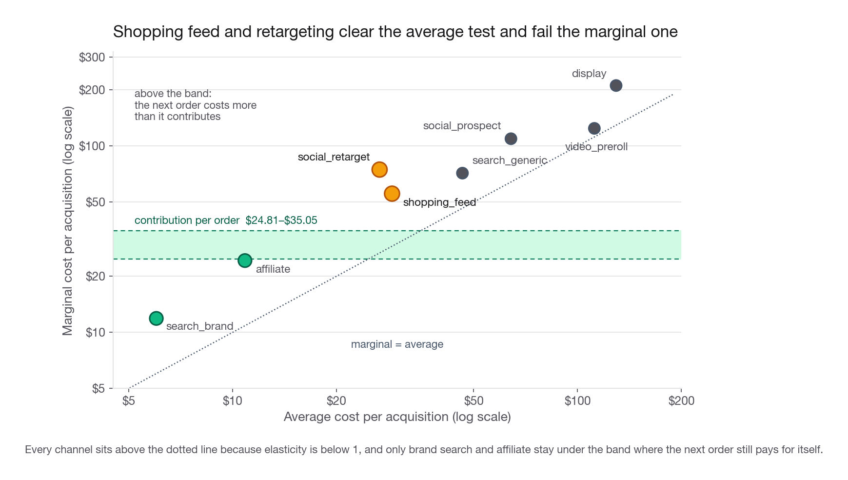
elasticity avg_cpa marginal_cpa contrib_per_order marginal_profit
search_brand 0.51 6.01 11.88 32.57 20.68
affiliate 0.45 10.86 24.28 28.35 4.07
shopping_feed 0.52 28.99 55.52 30.37 -25.16
social_retarget 0.36 26.68 74.74 35.05 -39.69
search_generic 0.65 46.38 71.53 30.01 -41.52
social_prospect 0.59 64.12 109.44 27.19 -82.25
video_preroll 0.90 111.89 124.39 25.90 -98.50
display 0.61 129.37 211.17 24.81 -186.35Read the two middle rows against the previous table. On average contribution, shopping feed and retargeting were both profitable, at 22,405 and 81,321 dollars. The fit says both are underwater at the margin: it puts the next shopping-feed order at 55.52 dollars against 30.37 of contribution, and the next retargeting order at 74.74 against 35.05. Four channels looked profitable on averages, two on this fit. That is where most submissions stop. Before you move a budget on it, check whether the slope is measuring the thing you named it after.
Two honesty requirements come with this method, and stating them unprompted is worth as much as the fit.
First, this elasticity is descriptive, not causal. Spend and orders both trend upward over 100 days, and anything else moving with time, seasonality, a redesign, a promotion, is bundled into the slope. It describes the path the team walked, not what happens if you change spend and hold everything else fixed. Say that, then say what fixes it: a staggered budget change across matched geographies, or at minimum a fit with a time control.
Second, the slope is only as stable as the channel's order volume and the range of spend it was estimated over. Bootstrap it before you build a recommendation on it.
def boot_elasticity(x, n=2000, seed=7):
    rng2 = np.random.default_rng(seed)
    out = np.empty(n)
    lx, ly = np.log(x.spend_usd.values), np.log(x.orders.values)
    for i in range(n):
        idx = rng2.integers(0, len(lx), len(lx))
        out[i] = np.polyfit(lx[idx], ly[idx], 1)[0]
    return np.percentile(out, [2.5, 97.5])

sub = d[(d.channel == "shopping_feed") & (d.orders > 0)]
print(np.round(boot_elasticity(sub), 3))
[0.416 0.626]For shopping feed that interval maps to a marginal cost per acquisition between 46.32 and 69.76 dollars, against contribution per order of 30.37. The tempting sentence here is that the whole interval sits above the bar, so the conclusion is robust. Do not write it. A bootstrap resamples rows from one specification, so it prices sampling noise inside that specification and is blind to the specification itself. It says nothing about the confounding this step already named, which the next block shows is the larger term by far.
Affiliate gives 0.379 to 0.513, straddling the bar. Display gives minus 0.12 to 1.33, a slope not identified at all on six orders a day. Both intervals are honest about sampling noise and both are about to be overtaken by a bigger problem.
Interview tip: Before you lean on a confidence interval, say out loud what it does not cover. It prices sampling noise around one specification, so if you have just called that specification confounded, the interval is the smaller of your two error sources.
Is that slope diminishing returns, or is it a price trend?
Spend is clicks times cost per click, so log spend carries two moving parts and only one of them is buying more inventory. Regress orders on clicks instead, fit the cost-per-click trend beside it, and add the time control this step promised.
t0 = d.date.min()
diag = []
for ch, x in d[d.click_ok & (d.orders > 0)].groupby("channel"):
    day = (x.date - t0).dt.days
    e_clicks = np.polyfit(np.log(x.clicks), np.log(x.orders), 1)[0]
    e_time = np.linalg.lstsq(np.column_stack([np.ones(len(x)), np.log(x.spend_usd), day]),
                             np.log(x.orders), rcond=None)[0][1]
    cpc_trend = np.polyfit(day, np.log(x.spend_usd / x.clicks), 1)[0]
    diag.append({"channel": ch, "on_spend": m.elasticity[ch], "on_clicks": e_clicks,
                 "spend_plus_time": e_time, "cpc_rise_pct": 100 * (np.exp(cpc_trend * 99) - 1)})
print(pd.DataFrame(diag).set_index("channel").round(2).to_string())
on_spend on_clicks spend_plus_time cpc_rise_pct
affiliate 0.45 0.94 0.76 53.00
display 0.61 1.45 1.06 30.89
search_brand 0.51 0.99 0.80 24.50
search_generic 0.65 0.95 0.73 38.52
shopping_feed 0.52 0.95 0.82 28.99
social_prospect 0.59 1.11 0.82 48.95
social_retarget 0.36 0.85 0.73 44.37
video_preroll 0.90 1.78 1.31 31.36That table takes the previous one apart. Orders track clicks close to one for one: the six channels with real volume land between 0.85 and 1.11, four inside 0.94 to 0.99, so nothing in these 100 days saturates. Cost per click meanwhile climbs 24 to 53 percent on every channel, while those same six ran only 0.36 to 0.65 against spend. That gap is what the spend slope was picking up: log spend rose partly because the team bought more clicks and partly because the same click got dearer, and the second half brings no orders with it. A linear time control pulls the slopes most of the way back toward 1, the same finding told twice.
So the marginal cost column above is not a marginal cost. It is an average cost inflated by a price trend the fit misread as diminishing returns.
What survives is narrower. If orders scale one for one with clicks and only price is moving, the next order costs what an order costs today, not what one cost on the 100-day average.
recent = d[d.date > d.date.max() - pd.Timedelta(days=30)]
r = recent.groupby("channel").agg(spend=("spend_usd", "sum"), orders=("orders", "sum"))
r["cpa_last_30d"] = r.spend / r.orders
r["contrib_per_order"] = m.contrib_per_order
r["margin_at_todays_prices"] = r.contrib_per_order - r.cpa_last_30d
print(r.drop(columns=["spend", "orders"]).round(2)
       .sort_values("margin_at_todays_prices", ascending=False).to_string())
cpa_last_30d contrib_per_order margin_at_todays_prices
search_brand 6.53 32.57 26.04
affiliate 12.68 28.35 15.67
social_retarget 31.09 35.05 3.96
shopping_feed 32.08 30.37 -1.71
search_generic 50.59 30.01 -20.58
social_prospect 71.53 27.19 -44.34
video_preroll 119.70 25.90 -93.81
display 135.74 24.81 -110.93Now correct the headline. Four channels looked profitable on 100-day averages and three still clear the bar at current prices. Shopping feed slips under by 1.71 dollars an order rather than the 25.16 the fit claimed, and retargeting is 3.96 ahead rather than 39.69 behind. Every dollar figure in Step 8 is sized off this table.
That reversal is the part of the write-up that earns the offer: you checked whether the regressor measured the thing you had named it after and said so before anyone asked. Keep the fit in the deck as a hypothesis with a test attached: step shopping-feed spend up 30 percent for four weeks and see whether orders follow one for one. Until somebody moves spend on purpose, the slope is not estimable from this path.
Step 6: Orders are not customers
Return on ad spend and cost per acquisition treat a repeat buyer identically to a first-time buyer. For a brand whose growth depends on the size of its customer base, that is the wrong unit for at least half the channels.
Assume a Kestrel customer places about 2.4 orders in year one at an average order value near 72 dollars. At 42 percent margin that is roughly 72.6 dollars of first-year contribution per new customer, the ceiling on what you can pay to acquire one under a twelve-month payback rule.
| Channel | New-buyer share of orders | New customers | Cost per new customer | Passes the 72.6 ceiling |
|---|---|---|---|---|
| search_brand | 28 percent | 13,016 | 21.39 | Yes |
| affiliate | 48 percent | 7,407 | 22.62 | Yes |
| shopping_feed | 44 percent | 7,142 | 65.96 | Yes |
| social_prospect | 81 percent | 7,022 | 79.28 | No, by 9 percent |
| search_generic | 55 percent | 11,317 | 84.92 | No |
| video_preroll | 73 percent | 744 | 152.95 | No |
| social_retarget | 17 percent | 1,640 | 158.04 | No, by a factor of 2.2 |
| display | 60 percent | 371 | 216.90 | No |
Two rows change the story. Retargeting, which looked like the third-best channel on return and was profitable on average contribution, buys new customers at 158 dollars because 83 percent of its orders come from people who already bought. It is a repeat-purchase channel wearing an acquisition channel's clothes, and judging it on cost per acquisition flatters it enormously. Prospecting social, which looked like a disaster at a return of 1.01, produced 7,022 of the 48,659 new customers in the window, 14.4 percent of all acquisition, at a cost only 9 percent above the ceiling.
Judge each channel on the job it actually does. Acquisition channels get measured on cost per new customer against first-year contribution. Retargeting gets measured on incremental orders against a holdout, because its entire value claim is that the order would not have happened otherwise, and that claim is untestable from this table.
Step 7: The attribution caveats that make the naive ranking wrong
Everything so far has taken the orders column at face value. That column is a credit assignment, not a measurement, and understanding how the credit was assigned changes the answer more than any modelling choice in this lesson.
Four specific distortions are visible in Kestrel's numbers.
The conversion window is same-day, as the schema note said. An order counts only if click and purchase land on the same calendar day. Housewares are a considered purchase: a shopper sees a video ad on Sunday, browses Tuesday, buys Friday, and the Sunday video gets nothing. This bias is not uniform. It falls almost entirely on the top of the funnel, exactly the four channels the naive ranking wants to cut. Whatever display and video are truly worth, this table understates it by an amount this file cannot reveal.
Credit goes to the last touch. Somebody who saw three prospecting ads, then typed "kestrel goods" into a search box and clicked the brand ad, appears in this table as a brand-search order at a cost per acquisition of 6.01. Brand search is a toll booth on demand that other channels created. A return of 12.90 on brand search is close to meaningless as a statement about incremental value.
Brand search cannibalises organic. A meaningful share of brand clicks would have arrived through the free organic result had the paid ad not been sitting above it. Companies that run brand holdouts routinely find a large fraction of paid brand clicks is traffic they would have received anyway. You cannot estimate that from these columns, and saying so is the correct answer.
Impressions are free and clicks are billed. Display buys 131 million impressions for 80,470 dollars because its click-through rate is roughly one in a thousand. Any view-through effect is invisible in a click-credited table, a further reason the ranking is biased against display and video specifically.
Put together, the naive ranking overpays the bottom of the funnel and underpays the top, so the recommendation falling out of it, cut everything upper-funnel, is the one most likely to be quietly wrong. It is also self-reinforcing: cut prospecting, watch brand searches decline six weeks later, and the dashboard blames a soft quarter.
The one honest way out is an experiment, and proposing a concrete one separates a good answer from a great one. The cheapest design here is a geographic holdout: take 20 metropolitan markets, match on pre-period revenue trend and channel mix, randomly assign ten to zero prospecting spend for six weeks while ten continue unchanged, and measure total company revenue per market rather than channel-attributed revenue. That last clause is the point. The outcome must be a number the attribution system cannot touch.
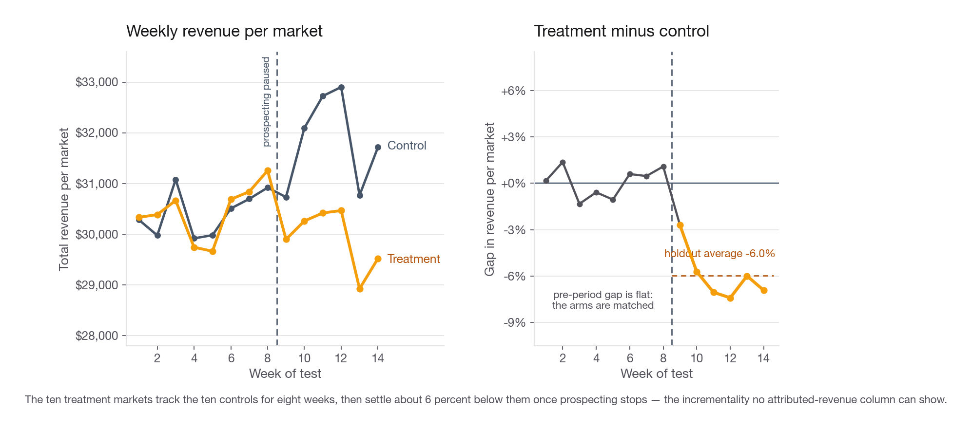
Size it before you propose it, and show the arithmetic, because the naive version of this design fails. With a coefficient of variation near 18 percent on market-level weekly revenue, ten markets per arm detects 2.80 times the square root of 2 over 10, times 0.18, which is 22.6 percent. Detecting a 6 percent drop that way needs 142 markets per arm and Kestrel does not have 142 markets. The design only survives if differencing against the pre-period strips that variance out. If week-to-week revenue inside a market moves by about 8 percent and the rest of the 18 percent is level differences between markets, six differenced weeks put the detectable effect near 6 percent, the same thing as a pre-and-post market correlation around 0.96. Check that split on pre-period data first, because differencing is not automatically a variance reduction: if the whole 18 percent were within-market noise, differencing gives 13.0 percent against 9.2 percent for a plain comparison of six-week means. At a correlation of 0.90 you see only 10.1 percent, and then you buy more markets, run longer, or write the larger number into the proposal.
Interview tip: Whenever you propose an incrementality test, name the outcome metric explicitly as total revenue rather than attributed revenue. Interviewers listen for that exact substitution.
Step 8: What to actually recommend
The deliverable is not the table, it is the reallocation. Here is the structure that lands, in the order a growth lead reads it.
Written out for Kestrel, with the numbers attached:
Scale affiliate, carefully. Besides brand it is the only channel with real headroom at today's prices: an order costs 12.68 and carries 28.35 of contribution. Do not read that gap as licence to double, because nothing here shows where affiliate saturates, so the increase is itself the measurement. Propose 25 percent, about 12,565 dollars a month, and re-read cost per order after four weeks.
Freeze shopping feed at current spend. It cleared break-even on average by 0.11 of return and sits 1.71 dollars an order underwater at today's cost per click, which is inside the noise. Do not cut it, do not grow it. Say plainly that a freeze leaves the elasticity unanswered, because only a deliberate spend step can answer it, and at 1.71 dollars an order that answer is not yet worth buying.
Hold retargeting and buy an answer instead. 259,192 dollars, 9 percent of budget. It clears break-even at 3.13, contributes 81,321, and is 3.96 dollars an order ahead at today's prices, so on unit economics it is neither a scale nor a cut. The deciding number is elsewhere: 83 percent of its orders come from people who already bought, cost per new customer is 158.04 against a 72.60 ceiling, and its whole value claim is that the order would not have happened anyway. Suppress it for a random half of the audience for four weeks and measure total orders per user.
Pull generic search back in stages. The largest lever: 961,027 dollars of spend, negative 339,201 of contribution, 20.58 dollars lost on every order at current prices. Solving the Step 5 fit for the spend where marginal cost equals 30.01 gives 828 dollars a day against 9,610 today, a 91 percent cut, and that answer sits at 16 percent of the lowest daily spend the channel has ever run. That is extrapolation outside the fitted range, a reason to distrust the fit rather than a cut order. Take 25 percent out, about 72,077 dollars a month, and watch whether cost per order falls as volume falls. If it does, the saturation curve is real. If not, take another 25 percent.
Run one upper-funnel holdout before touching prospecting or video. Extend the Step 7 geo design to pause video preroll in the same treatment markets. Together the two are 670,480 dollars, 23 percent of budget and 16.0 percent of new customers, and the same-day window damages both in the same direction. Cutting either on this table's numbers is the move most likely to be quietly wrong.
Cut display now. 80,470 dollars, 2.8 percent of budget, negative on average, 110.93 an order negative at today's prices, negative per new customer by a factor of three, and too small for a dedicated test to be worth the answer.
Test a brand-search budget reduction. Not a cut, a test. Reduce brand bids in half of the markets for four weeks and watch total revenue. Sized like the prospecting test, that sees about 7.3 percent, so read a flat result as "no cannibalisation bigger than 7 percent" rather than as proof the toll booth pays. If it is cannibalisation, you have found the largest saving in the portfolio.
Eight channels in, eight decisions out, and the dollars follow from the decisions.
| Channel | Monthly spend now | Decision | Monthly move |
|---|---|---|---|
| search_generic | 288,308 | Staged 25 percent pullback | -72,077 |
| display | 24,141 | Cut now | -24,141 |
| affiliate | 50,261 | Increase 25 percent | +12,565 |
| shopping_feed | 141,316 | Freeze | 0 |
| social_retarget | 77,758 | Hold, suppression holdout | 0 |
| social_prospect | 167,006 | Hold, geo holdout | 0 |
| video_preroll | 34,138 | Hold, same geo holdout | 0 |
| search_brand | 83,539 | Hold, bid-reduction test | 0 |
That is 96,218 dollars a month out of two channels and 12,565 back into one, a net 83,653 released from a monthly media budget of 866,467. Far smaller than the reallocation most candidates present, and defensible row by row. Five of the eight channels move nothing yet because three experiments come first: the upper-funnel geo holdout, the retargeting suppression test, and the brand-bid reduction. Saying "held pending experiments" instead of inventing a destination is the correct answer and the one most candidates are too nervous to give.
Common traps
Ranking on return on ad spend against a bar of 1.0. The bar is 1 divided by contribution margin. At 42 percent it is 2.381, and two of Kestrel's channels sit between 1.0 and 2.381: generic search at 1.54 and prospecting social at 1.01. That is the band where a channel clears the naive bar and still destroys money, 659,814 dollars of contribution between the two. The other two below break-even, video at 0.55 and display at 0.46, fail on any bar. Fix: compute break-even from margin early and put the line on every chart.
Averaging daily ratios. The mean of daily cost per acquisition overstates display's by 28 percent here, and on a channel with zero-order days it silently drops the worst days. Fix: aggregate numerator and denominator separately, then divide once.
Treating a renamed channel as two channels. The display migration to a new platform product split an 80,470-dollar channel into two rows that each looked too small to bother with. Fix: check the first and last date for every label before grouping.
Deleting anomalies without sizing them. Six negative revenue rows are worth 0.21 percent of revenue. Silent deletion is a habit that will, on a different dataset, delete the finding. Fix: quantify the impact before choosing the fix.
Counting a measurement outage as bad performance. Three consecutive zero-impression days on video are a broken pixel, not three dead days. Left in, they drag a daily average toward zero. Fix: separate "the ads did not work" from "we did not observe the ads", and handle spend and rates differently.
Recommending a scale-up from average return. A 100-day average says the money already spent worked, not what the next dollar does. Fix: compare contribution per order against cost per order over the most recent weeks, and reach for an elasticity only after checking that spend moved because volume moved rather than because price did.
Judging a retargeting channel on cost per acquisition. Retargeting shows a cost per acquisition of 26.68 and a cost per new customer of 158.04 because 83 percent of its orders are repeat buyers. Fix: match the metric to the channel's job, and demand a holdout for any channel whose claim is incrementality.
Cutting all four losing channels at once. They are 59.3 percent of spend and the top of the funnel that feeds brand search, whose 12.90 return is mostly harvested demand. Fix: separate channels you can cut on unit economics from channels whose measurement is structurally biased, and test the second group.
Treating a bootstrap as the whole error budget. The spend slope came from an observational path with a cost-per-click trend sitting inside the regressor, so a tight interval around it is false comfort: a bootstrap prices sampling noise within one specification and is blind to the specification. Fix: name the confounder, run the check that tests it, here orders on clicks against the cost-per-click trend, and only then ask whether the interval is the error term that matters.
Quick self-check
Answer these out loud, in full sentences, before you call the challenge finished.
Your contribution margin is 38 percent instead of 42. What is the break-even return on ad spend, which channels cross the line, and by how much does total portfolio contribution change?
A channel has an average cost per acquisition of 29 dollars, an elasticity of orders with respect to spend of 0.52, and an average order value of 72 dollars. What is the arithmetic that turns those into a marginal answer, and what would you have to check about the spend path before you trusted it?
Why does the same-day conversion window bias the ranking against display and video specifically, and how large would that bias have to be to reverse your recommendation on display?
You are told the eight channel order counts sum to 12 percent more than the company's actual order count. What does that tell you about the attribution setup, and which channel is most likely responsible?
Describe the geographic holdout you would run for prospecting social: number of markets, assignment, duration, outcome metric, and the smallest effect you could detect.
Retargeting has a cost per acquisition of 26.68 and a cost per new customer of 158.04. Which of those two numbers belongs in the recommendation, and what would you need to see before you cut the channel?