3.1 Challenge: Sessionizing Raw Event Logs
Find the core decision, design, or behavior signal.
Turn the lesson into a concise response blueprint.
Name the trap you would avoid in a real interview.
Use these checkpoints as your reading path before diving into the full lesson.
- 1What this lesson is for
- 2The brief
- 3Build the working copy
- 4Step 0: the integrity pass sessionizati...
- 5The sort is part of the definition
Dispatch is a news reading app. You open it on the train, read three or four stories, close it, come back that evening. The data team logs one row every time an article opens and nothing else. There is no session_id column because nobody ever wrote one. Product wants to know how many reading sessions a typical user has in a month and how long one lasts. Growth wants the same split by country, except a broken enrichment path leaves a quarter of the traffic carrying an empty country string, and it has been that way for as far back as this log goes. This lesson is the two judgment calls that decide your grade: where you cut one session from the next, and what you may claim about users whose country you cannot see.
What this lesson is for
Two skills get tested here and both are easy to fake badly.
The first is threshold defence. Sessionization needs a number, the inactivity gap, and no correct value is hiding in the data waiting to be found. A defensible value is: you show the distribution you read it off, show how much the answer moves when the threshold moves, and name the decision the number feeds. Writing gap = 30 minutes with no comment is not a mistake exactly, it skips the part being marked.
The second is inference from a behavioral fingerprint. You cannot look the missing country up. You reason from what people do and when, quantify it, name the candidates you cannot separate, and state a confidence that survives challenge. Most candidates handle this by squinting at a bar chart and asserting a continent.
Here is the weak submission in full: "I sessionized with a 30 minute gap. Users average 8.3 sessions per month and 149 seconds per session. The missing country is probably in Asia based on the activity hours." Every clause is true against this dataset. It scores badly because the grader cannot tell whether you know why.
The strong version says: the gap distribution is bimodal with a trough near 20 minutes, session counts move 2.8 percent across a 6x change in threshold so the choice is not load bearing, mean duration of 149 seconds is a floor rather than an estimate because the last page view has unobserved dwell time, and the unlabeled bucket sits at UTC plus 5.58 hours, 95 percent interval plus 5.33 to plus 5.84, which points at the plus 5:30 zone with a Saturday-Sunday weekend.
Interview tip: When a prompt hands you a parameter to choose, the answer they are marking is the sensitivity analysis, not the parameter.
The brief
Dispatch hands you one table, events, covering 28 days: roughly 100,000 rows across 4,000 users. One row is one article open.
| Field | Type | Notes |
|---|---|---|
event_id | int | Surrogate key, assigned on write, not meaningful |
user_id | int | Stable across devices, Dispatch requires login |
ts | timestamp, UTC | Server receive time, second resolution or better |
article_id | int | Which story was opened |
device | string | mobile or web |
country | string | Two letter code, or empty string for the affected cohort |
Three questions come with it.
Turn the raw log into sessions. State the inactivity gap you used and justify it from the data.
Report sessions per user and session duration. Give distributions, not just averages.
One country is not being logged at all. Which one, and how sure are you?
Question three is the one people remember and it is worth the least. One and two are where the interviewer learns whether you can be trusted with a table nobody has cleaned.
Build the working copy
Everything below runs against a synthetic log with the schema above. It is deterministic, so your numbers match the ones quoted here.
import numpy as np
import pandas as pd

SEED = 8240517
rng = np.random.default_rng(SEED)

OFFSET = {"US": -6.0, "GB": 0.0, "DE": 1.0, "BR": -3.0, "AU": 10.0, "": 5.5}
SHARE = {"US": 0.31, "GB": 0.14, "DE": 0.12, "BR": 0.09, "AU": 0.08, "": 0.26}
N_USERS, N_DAYS = 4000, 28
START = pd.Timestamp("2026-03-02", tz="UTC")  # a Monday

codes = list(OFFSET)
home = rng.choice(codes, size=N_USERS, p=[SHARE[c] for c in codes])
rows = []
for uid in range(1, N_USERS + 1):
    cc = home[uid - 1]
    for _ in range(1 + rng.poisson(9.0)):
        day = int(rng.integers(0, N_DAYS))
        if day % 7 >= 5 and rng.random() < 0.55:
            continue
        peak = 7.6 if rng.random() < 0.62 else 20.4
        local_h = rng.normal(peak, 1.5)
        t0 = START + pd.Timedelta(days=day, hours=float(local_h - OFFSET[cc]))
        n_ev = int(rng.geometric(0.34))
        gaps = np.concatenate([[0.0], rng.lognormal(3.9, 0.85, n_ev - 1)])
        for t in t0 + pd.to_timedelta(np.cumsum(gaps), unit="s"):
            rows.append((uid, cc, t))

events = pd.DataFrame(rows, columns=["user_id", "country", "ts"])
events["article_id"] = rng.integers(1000, 1400, len(events))
events["device"] = rng.choice(["mobile", "web"], len(events), p=[0.72, 0.28])
events = events.sort_values(["user_id", "ts"], kind="mergesort").reset_index(drop=True)
events["event_id"] = np.arange(1, len(events) + 1)
>>> len(events), events["user_id"].nunique()
(100363, 4000)
>>> events["country"].value_counts()
US 30141
26702
GB 15517
DE 11664
AU 8490
BR 7849The OFFSET dictionary knows the answer to question three. Cover that line until you have produced your own estimate from the timestamps, then use it to check yourself.
Note the empty-string bucket already: 26,702 events, second largest group, bigger than the United Kingdom. That framing belongs in your summary. This is not a rounding error, this is your number two market carrying no label at all.
Step 0: the integrity pass sessionization silently depends on
Sessionization is a sort, a diff, and a cumsum. All three inherit whatever is wrong with the input and none of them complain.
The sort is part of the definition
groupby(...).diff() differences against the previous row in the current row order. If the frame is not sorted by user and time the gaps are nonsense and nothing raises. Sort explicitly, immediately before the diff, even when you believe the frame is already sorted.
The folklore fix for ties is kind="mergesort", and it does nothing here. Pandas applies kind only when you sort on a single column or label; give by more than one key and it routes through lexsort_indexer, which is stable whatever you pass. So kind="mergesort" in sort_values(["user_id", "ts"], ...) is a no-op. Keep it for single-column sorts, where the quicksort default genuinely is unstable, and stop quoting it as the cure for ties.
A stable sort only means tied rows keep the order they arrived in, which does not make that order mean anything. Read the same events from a different file or a different partition and the ties arrive differently, so a different article gets credited as the session entry point. That is instability with respect to input order, not nondeterminism across runs: numpy's quicksort is introsort and returns the same permutation every time for the same array. Ties are not exotic on a second-resolution log: one tap firing a page view and a prefetch lands in the same second. What you need is a deterministic tiebreak column, so sort by ["user_id", "ts", "event_id"] and the order stops depending on how the rows arrived. Note that the build block above cannot do that, because event_id is numbered from its own output. On this frame the (user_id, ts) tie count is zero, so nothing quoted below moves, but that is a property of the data rather than of the sort.
Clock skew and negative gaps
Server receive time is usually monotone per user. Client emitted time is not. If the log ever mixes a client field with a server field you will see negative gaps, and gaps of exactly 3600 seconds clustered on daylight-saving transitions. Count them before you trust anything.
ev = events.sort_values(["user_id", "ts", "event_id"], kind="mergesort").copy()
ev["gap_s"] = ev.groupby("user_id")["ts"].diff().dt.total_seconds()
print("negative gaps:", int((ev["gap_s"] < 0).sum()))
print("exact-zero gaps:", int((ev["gap_s"] == 0).sum()))
print("gaps >= 28 days:", int((ev["gap_s"] >= 28 * 86400).sum()))
Zero gaps are the interesting case. They are duplicate emissions. A duplicate does not break sessionization, but it inflates events per session and deflates the mean inter-event time, which is the quantity you are about to use to pick the threshold. Decide whether a repeat open of the same article_id inside 2 seconds is one read or two, and dedupe on ["user_id", "ts", "article_id"] if the answer is one.
Bots wreck the gap estimate before they wreck anything else
A scraper hitting Dispatch every 45 seconds for six hours dumps a few thousand tightly spaced gaps into the region you are about to inspect. It barely moves the median, but it fills in the trough between the two modes and makes the threshold look less obvious than it is.
Screen cheaply: users whose gaps have a coefficient of variation near zero, users active in more than 20 distinct hours of the day, users above the 99.9th percentile on event count. Exclude them from threshold estimation even if you keep them in the reported metrics, and say so.
Interview tip: Say out loud which rows you excluded from choosing the threshold versus which rows you excluded from the final metric. Those are different decisions and graders check whether you know that.
Look for the onset of the blank country before you theorise about it
The empty country string is the headline of question three, so profile it here rather than in Step 4. The first thing to ask of any "a field stopped arriving" story is when it stopped.
d = events["ts"].dt.floor("D")
blank = events.groupby(d)["country"].apply(lambda s: 100 * (s == "").mean())
full = blank.loc["2026-03-02":"2026-03-29"]
print("daily blank share, min and max:", round(full.min(), 1), round(full.max(), 1))
print("first blank row:", events.loc[events["country"] == "", "ts"].min())
print("countries seen per user, max:", int(events.groupby("user_id")["country"].nunique().max()))
daily blank share, min and max: 21.9 31.7
first blank row: 2026-03-01 21:16:24.746422630+00:00
countries seen per user, max: 1There is no onset in this log. The blank share sits between 21.9 and 31.7 percent on every full day with no trend, by ISO week it is 27.0, 26.7, 26.4 and 26.6 percent, the first row of the log is already blank, and no user ever appears with both a code and a blank. This is a property of a fixed cohort of 1,055 users, not something that happened on a date.
Report the negative result, because of what it forecloses. There is no clean week in which the missing country still carries its code, so SELECT DISTINCT country on week one does not hand you the answer, and there is no bounded window to scope a backfill to. That is exactly why Step 4 has to reconstruct the country from behaviour instead of looking it up, and it belongs in the write-up, because otherwise a reader assumes you never checked.
Step 1: read the inter-event time distribution before choosing anything
The gap between consecutive events from one user is the only evidence you have about where sessions end. Look at it first.
Plot it on a log axis or you will see nothing
Gaps here run from about 1 second to about 20 days. On a linear axis that is one spike at zero and a screen of white space. On a log axis it is two clean humps.
import numpy as np

g = ev["gap_s"].dropna()
lg = np.log10(g.clip(lower=1))
counts, edges = np.histogram(lg, bins=np.arange(0, 6.2, 0.2))
for c, e in zip(counts, edges):
    print(f"{10**e:9.0f}s  {c:6d}  " + "#" * int(c / 400))
1s 10
2s 14
3s 103
4s 419 #
6s 1484 ###
10s 4025 ##########
16s 8029 ####################
25s 12513 ###############################
40s 14185 ###################################
63s 12227 ##############################
100s 7973 ###################
158s 3940 #########
251s 1437 ###
398s 475 #
631s 189
1000s 156
1585s 269
2512s 368
3981s 529 #
6310s 550 #
10000s 387
15849s 153
25119s 1564 ###
39811s 2624 ######
63096s 3755 #########
100000s 3003 #######
158489s 4755 ###########
251189s 5209 #############
398107s 3707 #########
630957s 1827 ####Two populations that barely touch. The left hump peaks in the 40 second bin at 14,185 gaps, a person finishing one article and tapping the next. The right hump peaks in the 251,189 second bin at 5,209, about three days, a person returning to the app. Between them, around 1,000 seconds, density falls to 156 gaps per bin, roughly a hundredth of the left peak. The thirty bins hold 95,879 of the 96,363 gaps; the other 484 run past 11.6 days and fall off the right edge, which is a churn question rather than a session question.
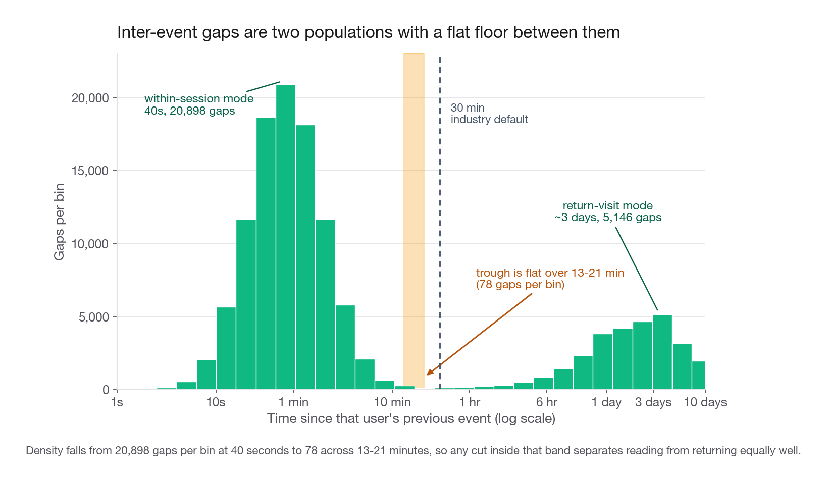
Quantiles say it in fewer numbers. The 65th percentile of the gap is 184 seconds, the 70th is 2,530 seconds, the 75th is 46,218 seconds. Nothing well behaved jumps by a factor of 14 between adjacent quantiles and then by another 18. That pair of jumps is the session boundary, and notice where it sits: about two thirds of all gaps are within-session, so the boundary is on the right shoulder of the first hump, nowhere near the median gap of 82 seconds.
The trough is the honest reading, and it is a range
Halve the bin width, 0.1 of a decade, and zoom on the 4 minute to 1 hour region:
z, edges_z = np.histogram(lg, bins=np.arange(2.4, 3.71, 0.1))
for c, e in zip(z, edges_z):
    print(f"{10**e:8.0f}s = {10**e/60:6.1f}min  {c:5d}")
251s = 4.2min 911
316s = 5.3min 526
398s = 6.6min 303
501s = 8.4min 172
631s = 10.5min 111
794s = 13.2min 78
1000s = 16.7min 78
1259s = 21.0min 78
1585s = 26.4min 123
1995s = 33.3min 146
2512s = 41.9min 169
3162s = 52.7min 199
3981s = 66.4min 257These counts run about half the ones above because the bins are half as wide, so read the shape and not the level. The minimum is flat across roughly 13 to 21 minutes, three consecutive bins at 78 apiece, and anywhere in there separates the two populations about equally well. That is more useful than a single number: the data cannot distinguish a 15 minute rule from a 20 minute rule, so do not pretend it does.
The 30 minute industry default sits just past the trough on the right shoulder. It is not wrong. It costs a small number of merges, pairs of reads separated by 22 to 30 minutes glued into one, and whether that matters depends on what you do with the sessions next.
Sensitivity beats the trough
Now the part that earns marks. Recompute the whole answer at every candidate threshold and see how much moves.
def sessionize(frame, gap_seconds):
    f = frame.sort_values(["user_id", "ts", "event_id"], kind="mergesort").copy()
    d = f.groupby("user_id")["ts"].diff().dt.total_seconds()
    f["is_new"] = d.isna() | (d > gap_seconds)
    f["session_seq"] = f.groupby("user_id")["is_new"].cumsum()
    f["session_id"] = f["user_id"].astype(str) + "-" + f["session_seq"].astype(str)
    return f

for minutes in [1, 2, 5, 10, 20, 30, 60, 240, 1440]:
    s = sessionize(events, minutes * 60)
    agg = s.groupby("session_id").agg(n=("ts", "size"), t0=("ts", "min"), t1=("ts", "max"))
    dur = (agg["t1"] - agg["t0"]).dt.total_seconds()
    print(minutes, len(agg), round(len(agg) / s["user_id"].nunique(), 2),
round(dur.mean(), 1), round(100 * (agg["n"] == 1).mean(), 1))| Gap | Sessions | Sessions per user | Mean duration (s) | Single-event sessions |
|---|---|---|---|---|
| 1 min | 61,129 | 15.28 | 20.6 | 61.1% |
| 2 min | 43,598 | 10.90 | 62.7 | 43.7% |
| 5 min | 34,703 | 8.68 | 123.4 | 34.9% |
| 10 min | 33,572 | 8.39 | 140.7 | 33.6% |
| 20 min | 33,280 | 8.32 | 149.0 | 33.3% |
| 30 min | 33,127 | 8.28 | 156.6 | 33.2% |
| 60 min | 32,628 | 8.16 | 199.8 | 32.7% |
| 4 hours | 31,147 | 7.79 | 570.6 | 31.1% |
| 24 hours | 24,676 | 6.17 | 14,805.6 | 25.0% |
Read the middle of that table carefully. Between 10 and 60 minutes, a 6x change in threshold, session count moves 2.8 percent and sessions per user goes from 8.39 to 8.16. The metric is insensitive across the entire plausible range, which converts a subjective choice into a non-issue. Put that sentence in the write-up.
Below 5 minutes the count explodes and the single-event share doubles. Above 4 hours mean duration becomes meaningless, because a 24 hour rule glues a morning read and an evening read into one 15,000 second "session" nobody experienced.
So: 20 minutes, read off the trough, with a note that 10 to 60 tells the same story and under 5 does not.
Raise the fourth row verbally even when you cannot use it. If Dispatch is sizing push notification frequency, a session means "an app opening" and 20 minutes is right. If Dispatch bills advertisers per session, the contract already defines it and your opinion is irrelevant. Saying that is worth more than the estimate.
Interview tip: Never present a chosen threshold without the sentence "and here is how much the answer changes if I move it", with an actual number attached.
Step 2: sessionize, in pandas and in SQL
The pandas version is four lines and the trick is entirely in the boolean.
GAP_SECONDS = 20 * 60

ev = events.sort_values(["user_id", "ts", "event_id"], kind="mergesort").copy()
ev["gap_s"] = ev.groupby("user_id")["ts"].diff().dt.total_seconds()
ev["is_new"] = ev["gap_s"].isna() | (ev["gap_s"] > GAP_SECONDS)
ev["session_seq"] = ev.groupby("user_id")["is_new"].cumsum()
ev["session_id"] = ev["user_id"].astype(str) + "-" + ev["session_seq"].astype(str)
print(ev.head(6)[["user_id", "ts", "gap_s", "is_new", "session_seq"]])
user_id ts gap_s is_new session_seq
0 1 2026-03-03 00:24:28.839+00:00 NaN True 1
1 1 2026-03-03 00:25:15.028+00:00 46.19 False 1
2 1 2026-03-05 00:15:40.212+00:00 172225.18 True 2
3 1 2026-03-05 15:13:29.212+00:00 53869.00 True 3
4 1 2026-03-05 15:13:59.354+00:00 30.14 False 3
5 1 2026-03-08 21:28:00.898+00:00 281641.54 True 4Three details there belong in the write-up.
The first event of every user has a null gap, and isna() must be folded into is_new explicitly. Forget it and every user's first session merges into their second, silently, with no error and a plausible result.
The comparison is strictly greater than, so a gap of exactly 1,200 seconds continues the session. Either convention is fine, but the SQL and pandas paths must use the same one or your two answers will differ by a few hundred sessions and you will lose an hour finding out why.
The session key concatenates user_id with the per-user counter. Never use the bare counter: session 3 exists for every user, and joining on it produces a cross product that looks like a data quality problem for the rest of the afternoon.
The same logic in SQL
Warehouses do this with two window functions and a running sum. The version below runs on Postgres, BigQuery, Snowflake, or Redshift with only the timestamp arithmetic swapped, plus one cast: BigQuery's || takes strings and bytes only, so user_id || '-' || session_seq needs CAST around both integers there.
WITH flagged AS (
  SELECT
    user_id,
    ts,
    event_id,
    article_id,
    CASE
      WHEN LAG(ts) OVER (PARTITION BY user_id ORDER BY ts, event_id) IS NULL
        THEN 1
      WHEN EXTRACT(EPOCH FROM ts - LAG(ts) OVER (
             PARTITION BY user_id ORDER BY ts, event_id)) > 1200
        THEN 1
      ELSE 0
    END AS is_new
  FROM events
),
keyed AS (
  SELECT
    user_id, ts, article_id,
    SUM(is_new) OVER (PARTITION BY user_id ORDER BY ts, event_id
                      ROWS BETWEEN UNBOUNDED PRECEDING AND CURRENT ROW) AS session_seq
  FROM flagged
)
SELECT
  user_id,
  user_id || '-' || session_seq AS session_id,
  MIN(ts) AS started_at,
  MAX(ts) AS ended_at,
  COUNT(*) AS events,
  COUNT(DISTINCT article_id) AS articles,
  EXTRACT(EPOCH FROM MAX(ts) - MIN(ts)) AS duration_s
FROM keyed
GROUP BY user_id, session_seq;
Say the frame clause out loud when you present this, and say the ordering key in the same breath, because they are one decision. The default frame on an ordered window is RANGE BETWEEN UNBOUNDED PRECEDING AND CURRENT ROW, and RANGE includes every peer row tying on the ordering expression. Two events at the same timestamp are peers, so both get the same running sum and a boundary landing on a tie applies to both at once. That is a known-wrong answer.
ROWS only fixes it once the ORDER BY is a total order. Under ORDER BY ts alone it hands each tied row a different running sum in an order the engine is free to choose, so a boundary on a tie can glue the second tied row onto the session that ended an hour earlier: a known-wrong answer traded for an unstable one. That is why event_id appears in both windows and why flagged has to project it. Inline the CTEs and the planner often reuses the LAG's sort and hides the problem; materialize the intermediate step, which the cost section below tells you to do anyway, and it stops hiding.
The warehouse gotchas that cost real money
Partitioning by user_id and ordering by ts forces a full shuffle on the user key. On a few hundred million events that shuffle is the dominant cost of the pipeline, so materialize sessions once a day instead of sessionizing inside every downstream query.
Sessions cross midnight and cross partition boundaries. If the table is partitioned by date and you process one day at a time, every session starting at 23:52 gets split. Read a lookback of one day plus the gap, then discard sessions whose first event falls outside the target day.
BigQuery has SESSION_WINDOW and Snowflake has CONDITIONAL_TRUE_EVENT. Use them if the warehouse is fixed, but be able to write the portable version, because that is what is being checked.
Interview tip: If you write the window function version, name the frame clause and why it isROWSand notRANGE. It takes one sentence and it is the single clearest signal that you have shipped this before.
Step 3: sessions and durations per user
With sessions in hand the aggregation is routine. What duration means is not.
sessions = (ev.groupby(["session_id", "user_id", "country"], as_index=False)
              .agg(started_at=("ts", "min"), ended_at=("ts", "max"),
                   events=("event_id", "size"), articles=("article_id", "nunique")))
sessions["duration_s"] = (sessions["ended_at"] - sessions["started_at"]).dt.total_seconds()

per_user = (sessions.groupby(["user_id", "country"], as_index=False)
                    .agg(sessions=("session_id", "size"), events=("events", "sum"),
                         total_s=("duration_s", "sum"), median_s=("duration_s", "median")))
print(len(sessions), round(per_user["sessions"].mean(), 2))
33280 8.32The single-event session is the whole problem
A third of sessions here, 33.3 percent, contain exactly one event, so under a last-minus-first definition their duration is zero seconds. That is not a measurement, it is an artifact of the definition, and it drags median session duration to 66 seconds against 147 seconds among multi-event sessions.
Reporting "median session duration is 66 seconds" is defensible only if you say in the same breath that a third of sessions are single reads with unobservable duration. Without that sentence it gets caught in the follow-up and unwinds the rest of your credibility. Three honest options and one dishonest one:
| Approach | What it reports | When it is right | Risk |
|---|---|---|---|
| Last minus first, keep zeros | 149.0 s mean, 66.4 s median | Comparing session length across cohorts on the same definition | Reads as "users spend no time" to a non-technical reader |
| Last minus first, multi-event only | 223.5 s mean, 146.9 s median | Describing what a reading session looks like when it happens | Silently drops a third of sessions, must be labeled |
| Add an imputed final dwell | 179.0 s mean at 30 s imputed | Estimating total time on app, where the tail matters | The imputed constant is an assumption, needs a sensitivity check |
| Drop singletons and say nothing | Whatever it says | Never | This is the one that gets you rejected |
Do the imputation properly, because the sensitivity is large. Total measured reading time over 28 days is 1,378 hours with no imputation, 1,563 at 20 seconds, 1,655 at 30, and 1,932 at 60. That is a 40 percent spread driven entirely by a constant you invented. Anyone quoting "hours read per month" in a board deck needs to know that.
If Dispatch logs an article-close or a scroll-depth ping, use it and the problem disappears. Ask. "Does the client emit a heartbeat while an article is open" is a strong live question, because it shows you know gap-measured duration is a workaround for missing instrumentation rather than a definition of engagement.
What to report
Distributions, not centres. Sessions per user over 28 days:
| Statistic | Sessions per user | Events per user | Total duration (s) |
|---|---|---|---|
| p10 | 5 | 12 | 393 |
| p25 | 6 | 17 | 685 |
| median | 8 | 24 | 1,105 |
| p75 | 10 | 31 | 1,663 |
| p90 | 12 | 40 | 2,242 |
| max | 19 | 77 | 5,117 |
Sessions per user is tight, p10 of 5 to p90 of 12, which is itself worth a sentence: Dispatch has no power-user tail on visit frequency, unlike most consumer apps. Events per user spans 12 to 40, four times the spread. People differ far more in how much they read per visit than in how often they visit. Report only means and that contrast vanishes, along with the most interesting line in the analysis.
Three users have exactly one session in 28 days. Check them rather than assuming they are bugs, and notice what checking actually settles. Their single sessions land on 9, 11 and 15 March, days 7, 9 and 13 of the window, so the story that leaps to mind, that they signed up near the end, is ruled out by the data in front of you. Those sessions carry 4, 1 and 7 events, which read as ordinary short visits rather than instrumentation failures. What you cannot settle from this table is why they are so quiet, because events carries no signup date. Say that out loud rather than filling the hole with a guess: the answer is a join to a users table with a created_at, and until you have it, a genuinely low-frequency reader and a late joiner are indistinguishable here.
Step 4: the country that is not being logged
Now the detective question. You have 26,702 events, 8,905 sessions, and 1,055 users with an empty country string, no lookup, and timestamps. The chain of reasoning is short and every link is testable.
First, test whether it is one population
If the enrichment failure hit one country, the empty bucket is a single population and should look like one. If it hit every Android user on a version older than 4.2, the bucket is a mixture of every country and should look smeared.
The clean test is how concentrated the activity is around the clock. Convert each session start to an angle on a 24 hour circle and compute the mean resultant length R, which runs from 0 for uniform to 1 for everything at one instant.
def circular_stats(minutes_of_day):
    theta = 2 * np.pi * np.asarray(minutes_of_day) / 1440.0
    c, s = np.cos(theta).mean(), np.sin(theta).mean()
    angle = np.arctan2(s, c) % (2 * np.pi)
    return angle / (2 * np.pi) * 1440.0, np.hypot(c, s)

sessions["mod"] = sessions["started_at"].dt.hour * 60 + sessions["started_at"].dt.minute
for code, grp in sessions.groupby("country"):
    mean_min, R = circular_stats(grp["mod"])
    print(f"{code or '(blank)':>8}  mean {int(mean_min)//60:02d}:{int(mean_min)%60:02d}  R={R:.3f}  n={len(grp)}")
(blank) mean 00:57 R=0.247 n=8905
AU mean 20:28 R=0.246 n=2797
BR mean 09:35 R=0.247 n=2679
DE mean 05:35 R=0.259 n=3840
GB mean 06:32 R=0.248 n=5073
US mean 12:24 R=0.234 n=9986The blank bucket has R = 0.247, inside the labeled range of 0.234 to 0.259. Now build the contrast properly, by pooling labeled countries into fake mixed buckets and asking what a mixture actually costs.
def pooled_R(codes):
    m = sessions["country"].isin(codes)
    return circular_stats(sessions.loc[m, "mod"])[1]

for pair in [["US", "AU"], ["US", "DE"], ["BR", "US"], ["GB", "DE"]]:
    print(f"{'+'.join(pair):>8}  R={pooled_R(pair):.3f}")
print(f"all five  R={pooled_R(['US', 'GB', 'DE', 'BR', 'AU']):.3f}")
US+AU R=0.162
US+DE R=0.170
BR+US R=0.226
GB+DE R=0.251
all five R=0.128The tidy version of this test is a trap, so read the floor as well as the headline. Two widely separated zones do collapse: the US with Australia, eight hours apart, pools to 0.162, the US with Germany to 0.170. But Brazil with the US, under three hours apart, pools to 0.226, and Britain with Germany, one hour apart, pools to 0.251, higher than the US on its own and comfortably inside the labeled range. By three hours of separation the signal is already marginal, and by one hour it is gone. Say "low dispersion proves a single country" and you get handed that counterexample.
What R does rule out is the alternative on the table. A failure tied to an app version would make the blank bucket a thin slice of every market, which is what pooling all five labeled countries models: 0.128. The blank bucket at 0.247 is nowhere near it.
That is claim one, quantified and stated no more strongly than the evidence allows: the unlabeled traffic sits in one narrow band of longitudes, not smeared across every market. It does not yet rule out two neighbours sharing a clock. The calendar step below is what narrows that.
Estimate the offset, not the peak hour
Most candidates find the modal hour and count how far it sits from a known country's modal hour. That gets you the nearest hour on a good day. The mean of the whole distribution does better, because it uses every event instead of the tallest bar.
Local behaviour is the same everywhere in this product, a commute peak and an evening peak, so mean local session time is the same constant for every country and mean UTC time is that constant minus the offset. Anchor on a country whose offset you know, take differences, and the constant cancels.
def offset_vs(anchor_code, target_code, frame):
    a, _ = circular_stats(frame.loc[frame["country"] == anchor_code, "mod"])
    b, _ = circular_stats(frame.loc[frame["country"] == target_code, "mod"])
    hours = (a - b) / 60.0
    return (hours + 12) % 24 - 12

for code in ["US", "BR", "DE", "AU", ""]:
    print(f"{code or '(blank)':>8}  implied UTC{offset_vs('GB', code, sessions):+.2f}h")
US implied UTC-5.87h
BR implied UTC-3.06h
DE implied UTC+0.94h
AU implied UTC+10.05h
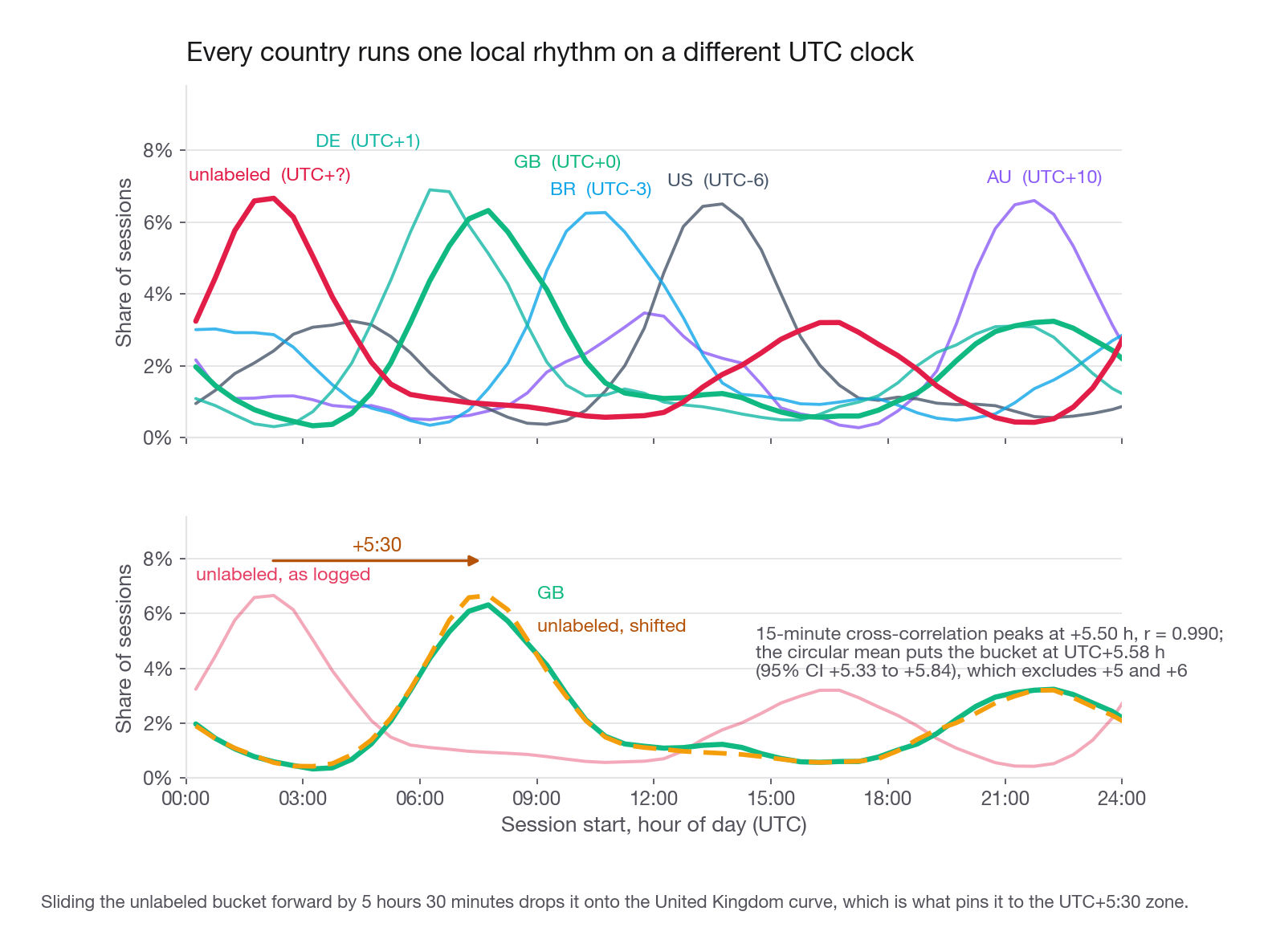
(blank) implied UTC+5.58hValidate the method before trusting its output. The known countries come back at minus 5.87, minus 3.06, plus 0.94, and plus 10.05, against truths of minus 6, minus 3, plus 1, and plus 10. The estimator is good to about a tenth of an hour at these sample sizes, so the plus 5.58 for the blank bucket now means something: the ruler is calibrated.
Bootstrap it so you can exclude candidates instead of merely ranking them. Resampling anchor and target 2,000 times gives plus 5.58 hours, 95 percent interval plus 5.33 to plus 5.84.
Half-hour offsets are a fingerprint
That interval is the whole answer, and it is worth pausing on why.
Almost every zone on earth is a whole number of hours from UTC. The exceptions are a short list: plus 5:30, plus 5:45, plus 4:30, plus 3:30, plus 9:30, plus 6:30, minus 3:30, plus 8:45, plus 12:45. An interval of plus 5.33 to plus 5.84 excludes plus 5:00 and plus 6:00 by comfortable margins and lands on plus 5:30, with plus 5:45 the only serious alternative.
Confirm with a second, shape-free method so the conclusion does not rest on a circular mean being appropriate for a bimodal distribution. Bin both profiles into 15 minute buckets, roll one against the other, and find the lag that maximises correlation.
bins = np.arange(0, 1441, 15)
def profile(codes_mask):
    h, _ = np.histogram(sessions.loc[codes_mask, "mod"], bins=bins)
    return h / h.sum()

ref = profile(sessions["country"] == "GB")
tgt = profile(sessions["country"] == "")
scores = [(k * 15 / 60, float(np.corrcoef(ref, np.roll(tgt, k))[0, 1])) for k in range(96)]
for lag, r in sorted(scores, key=lambda x: -x[1])[:4]:
    print(f"lag {lag:5.2f}h  r={r:.4f}")
lag 5.50h r=0.9903
lag 5.75h r=0.9768
lag 5.25h r=0.9763
lag 6.00h r=0.9458The best alignment is exactly 5.50 hours with a correlation of 0.990. Be careful how hard you lean on that. One bin either side sits at 0.977 and 0.976, so the cross-correlation ranks plus 5:30 first, it does not exclude its neighbours; the fall-off only becomes decisive by plus 6:00, at 0.946. Two independent methods, one parametric on the circle and one a plain cross-correlation of the raw profile, put the peak in the same place, and that is worth saying. What neither of them does is separate plus 5:30 from plus 5:45. That is the next step, not a detail to wave past.
The calendar rules out the rest
Plus 5:30 is India and Sri Lanka. Plus 5:45 is Nepal. Population and English-language news consumption make India the likely source of a bucket this size, but that is a prior, not evidence, so go find evidence.
The working week separates zones that share a clock. Shift into estimated local time first, because running weekday analysis in UTC is exactly the mistake this exercise is built to catch.
shifted = sessions.loc[sessions["country"] == ""].copy()
local = shifted["started_at"] + pd.Timedelta(hours=5.5)
names = ["Mon", "Tue", "Wed", "Thu", "Fri", "Sat", "Sun"]
share = local.dt.dayofweek.value_counts(normalize=True).sort_index() * 100
print({names[i]: round(v, 1) for i, v in share.items()})
{'Mon': 16.9, 'Tue': 17.3, 'Wed': 16.8, 'Thu': 16.7, 'Fri': 16.6, 'Sat': 8.1, 'Sun': 7.5}Five weekdays at 16.6 to 17.3 percent each, then a clean halving on Saturday and Sunday. That rules out two things at once, and the second is the one that earns its keep. A working week running Sunday to Thursday, the Gulf pattern, would leave Sunday busy and Friday quiet, and the data says the opposite. And Nepal, the plus 5:45 candidate, runs Sunday to Friday with Saturday as its single weekly holiday, so a Nepali bucket would put Sunday near 16 percent with only Saturday depressed. Sunday is at 7.5 percent. That kills plus 5:45, which the offset interval could not: plus 5.33 to plus 5.84 contains plus 5.75, and the cross-correlation only ranked it second. Check that the test is not circular before you use it, because it would be easy for it to be: recompute the shares shifting by plus 5.75 instead of plus 5.5 and you get Saturday 8.1 and Sunday 7.5 again, so the calendar reading does not depend on which of the two zones you assume.
Look at what the local-time correction bought you. Australia's raw UTC weekday profile shows Friday at 10.9 percent and Sunday at 13.5 percent, a bizarre calendar until you remember that plus 10 hours pushes Australian evenings into the previous UTC day. Shifted to local, Australia has the same clean weekend trough as everyone else. Run the same test in UTC on a real market and you conclude something false about it.
Interview tip: Any day-of-week claim about an international user base is wrong until you have converted to local time, and the conversion requires the offset you just estimated, so the order of operations is not optional.
Writing the answer
Here is the paragraph. It leads with the conclusion, carries its uncertainty, and ends with the action.
The unlabeled bucket sits in one narrow band of longitudes, not smeared across every market: its activity concentration, R of 0.247, matches labeled single countries at 0.234 to 0.259, while a thin slice of all five labeled markets pools to 0.128. Its clock sits at UTC plus 5.58 hours, 95 percent interval plus 5.33 to plus 5.84, and a 15 minute cross-correlation against the United Kingdom profile peaks at exactly plus 5.50 with r of 0.99. That excludes plus 5 and plus 6, but not plus 5:45, because the interval contains it. The calendar settles that one: in local time the traffic halves on both Saturday and Sunday, and Nepal, the plus 5:45 candidate, works Sunday to Friday with Saturday as its only weekly holiday, so a Nepali bucket would show a normal Sunday. What is left is plus 5:30, which means India or Sri Lanka, and these timestamps cannot separate those two at all: they share a clock and a weekend. India over Sri Lanka rests on the bucket being 26 percent of all events against Sri Lanka being roughly a sixtieth of India's population, which is a prior on market size and not something the log shows. So: high confidence on the zone off the clock and the calendar, high confidence on India carried by that prior rather than by the data. The fix is a schema check on the country enrichment path, and the field should be backfilled by joining on IP geolocation across the whole log, since every row this cohort ever emitted is affected, rather than written from this inference.
That last clause matters. You have identified the country well enough to tell an engineer where to look, not well enough to write into the warehouse as fact. Saying so is the difference between an analyst and someone who eventually corrupts a table.
What sessionization changes downstream
Two consequences belong in the write-up, because they show you know the artifact has a life after you hand it in.
Session-level metrics are not event-level metrics with a groupby in front. Click-through rate per session and per event move in opposite directions when session length changes. Ship a feature that lengthens sessions and per-session engagement rises while per-event engagement falls, and both are correct.
Freeze the gap before an experiment and never change it mid-flight. Switching from 30 minutes to 15 halfway through a test moves sessions per user about 1 percent and mean duration about 5 percent, and a team will spend a week attributing that to the treatment. Put the gap in the metric definition doc next to the metric name.
Common traps
Choosing 30 minutes because everyone does. The number is fine here, the missing justification is what costs marks. Show the trough and the sensitivity table, then use 30 minutes if you like.
Diffing an unsorted frame.
groupby().diff()uses row order, not time order, and produces plausible garbage with no warning. Sort by user, timestamp, and event id immediately before the diff, every time.Dropping the first-event null. A null gap must be treated as a session start. Omit it and every user's first session merges into their second, silently.
Using a bare per-user session counter as a key. Session 4 exists for thousands of users, so any join on it explodes. Prefix with the user id.
Reporting median duration without the singleton share. It is 66 seconds overall and 147 seconds among multi-event sessions. Quoting the first without the 33 percent context is misleading, and the follow-up will find it.
Treating an imputed final dwell as data. A 30 second assumption moves total reading hours by 20 percent. Show the sensitivity, and never let the number leave your analysis without its assumption attached.
Reading the missing country off the modal hour. The mode gives you the nearest hour at best. The circular mean of every event resolves half-hour offsets, which is what actually identifies the zone.
Doing day-of-week analysis in UTC. Past plus 8 or below minus 6 the UTC weekday profile is a shifted smear of the real one. Convert first.
Stating the country as a fact. You have a time zone and a weekend pattern. Say plus 5:30 with high confidence off the clock and the calendar, say India with high confidence but name the volume prior it rests on, name Sri Lanka as the candidate your timestamps cannot separate, and recommend the engineering check rather than a warehouse backfill from your inference.
Reading a low R as proof of a single country. It rules out a broad multi-market smear, not two neighbours sharing a clock. Britain pooled with Germany gives 0.251 and sails through the test. Say what the statistic excludes, which is the app-version story at 0.128, not what it cannot see.
Theorising about a missing field without checking when it went missing. Plot the blank share by day first. Here it is flat from the first row of the log, which kills the "look it up in the week before the breakage" shortcut and is the reason the rest of Step 4 exists.
Sessionizing inside every downstream query. The partition-and-order shuffle is the expensive part. Materialize once, with a lookback so midnight-crossing sessions are not split.
Ignoring bots when estimating the threshold. A scraper on a fixed interval fills the trough and makes a clean bimodal distribution look ambiguous.
Quick self-check
Answer out loud, in full sentences, as if the interviewer just asked.
Your inter-event gaps have a 65th percentile of 184 seconds and a 70th percentile of 2,530 seconds. What does that tell you, and what would you conclude instead if the two were 184 and 260?
Session count changes by 2.8 percent between a 10 minute and a 60 minute gap. What does that let you stop worrying about, and what does it specifically not let you stop worrying about?
A third of your sessions have exactly one event and therefore a duration of zero. Give three defensible ways to report duration and name the situation each one is right for.
You estimate the unlabeled bucket at UTC plus 5.58 hours with a 95 percent interval of plus 5.33 to plus 5.84. Which candidate zones does that exclude, which does it fail to exclude, and what non-clock evidence would you reach for next?
R for the unlabeled bucket is 0.247, inside the labeled single-country range. What alternative does that rule out, what kind of mixture would still pass it, and what value would you expect instead if the logging failure were tied to an app version rather than to a country?
Your window function uses
ROWS BETWEEN UNBOUNDED PRECEDING AND CURRENT ROW. What breaks if you leave the frame clause off, what breaks differently if you keep it but order only byts, and under what data condition does either breakage actually show up?