5.2 Challenge: Measuring a Referral Program
Find the core decision, design, or behavior signal.
Turn the lesson into a concise response blueprint.
Name the trap you would avoid in a real interview.
Use these checkpoints as your reading path before diving into the full lesson.
- 1Why this matters in interviews
- 2The brief you were handed
- 3Step 1: Reconcile the file before you t...
- 4The referral flag lives on the wrong grain
- 5Two populations that cannot exist
A growth manager at Munch, a food delivery app, launched a referral program and signups jumped. She wants a number she can put on a slide for her director by Friday. There was no randomization: the program went live in four metros on one day, for everyone in those metros at once. Your job is to decide how much of that jump the program actually caused, how much of it is worth anything, and how loudly you are allowed to say so. This lesson walks the whole path, from the broken flag in the export to the sentence you put at the top of the deck.
Why this matters in interviews
Every company runs launches like this. Somebody ships a feature to everyone on a Tuesday and then asks what it did. The honest answer requires a comparison group you were not given, and constructing one is the single most transferable skill in applied analytics.
Interviewers use this challenge because it separates three tiers of candidate cleanly.
The bottom tier computes the before-and-after change and reports it. They will tell you signups rose 23.5 percent and stop. They are not wrong about the arithmetic, they are wrong about what the arithmetic means.
The middle tier knows the phrase "difference in differences", builds a comparison group, runs the regression, and reports a smaller number with a confidence interval. This is competent and gets you a callback at most places.
The top tier does all of that and then asks the question the growth manager did not: of the accounts the program attracted, how many are new humans, how many are people who were going to sign up anyway and simply routed through a friend's link to get a discount, and how many are the same person opening a second account on the same phone to harvest their own credit. Then they price all three and tell the manager whether to keep the program. That candidate gets the offer.
Interview tip: The sentence "the program is credited with 16,934 signups, and I estimate about 3,000 of them would not have happened otherwise" is the whole interview in one line. Practice saying it without hedging.
The brief you were handed
Munch operates in eight metros. On 2026-04-15 the referral program went live in four of them: Alder, Birchwood, Cormont, and Dunfield. An existing customer shares a link, and when the invited person completes their first paid order, the inviter receives 12 in Munch credit. The other four metros, Elmsgate, Fenwick, Grayling, and Holloway, were left alone because the operations team wanted to stagger the support load. Nobody thought of this as an experiment. It is the only reason the question is answerable.
You get one table, one row per order, covering 2026-03-01 through 2026-05-31.
| Column | Type | What it holds |
|---|---|---|
order_id | int | Unique order key |
user_id | int | Account that placed the order |
order_date | date | Delivery date |
market | text | One of the eight metros |
order_value | float | Basket total in dollars, before credits |
is_referred | int | 1 if the account was acquired through a referral link |
device_hash | text | Fingerprint of the device used to place the order |
The block below builds that table deterministically. Every figure quoted for the rest of this lesson comes out of it, including the defects, which were planted because real exports have them.
import numpy as np
import pandas as pd

SEED = 20260415
rng = np.random.default_rng(SEED)
MARKETS = ["Alder", "Birchwood", "Cormont", "Dunfield",
           "Elmsgate", "Fenwick", "Grayling", "Holloway"]
TREATED = MARKETS[:4]
START, DAYS, LAUNCH = pd.Timestamp("2026-03-01"), 92, 45
size = dict(zip(MARKETS, [1.00, .82, .66, .51, .93, .74, .60, .46]))
d = np.arange(DAYS)
season = 1 + 0.17 * (((d + 5) % 7) >= 5) + 0.0034 * d
parts = []
for m in MARKETS:
    w = season * (1 + 0.082 * ((d >= LAUNCH) & (m in TREATED)))
    parts.append(pd.DataFrame({"market": m,
                               "join_day": np.repeat(d, rng.poisson(190 * size[m] * w))}))
u = pd.concat(parts, ignore_index=True)
u["user_id"] = 500000 + rng.permutation(len(u))
u["referred"] = rng.random(len(u)) < np.where(
    (u.join_day >= LAUNCH) & u.market.isin(TREATED), 0.46, 0.0)
u["farm"] = u.referred & (rng.random(len(u)) < 0.31)
u["device_hash"] = np.array(["D%08d" % i for i in rng.integers(0, 90_000_000, len(u))])
u.loc[u.farm, "device_hash"] = rng.choice(u.device_hash[~u.referred].values, u.farm.sum())
k = np.where(u.farm, 1, 1 + rng.poisson(np.where(u.referred, 0.85, 1.55)))
o = u.loc[np.repeat(u.index.values, k)].reset_index(drop=True)
o["seq"] = o.groupby("user_id").cumcount()
o["day"] = o.join_day + o.seq * rng.integers(3, 16, len(o))
o = o[o.day < DAYS].reset_index(drop=True)
n = len(o)
o["order_value"] = np.round(np.where(o.farm, rng.gamma(3.1, 2.6, n),
                            rng.gamma(6.4, np.where(o.referred, 3.4, 4.2), n)), 2)
o["is_referred"] = o.referred.astype(int)
flip = rng.random(n) < 0.012
o.loc[flip, "is_referred"] = 1 - o.loc[flip, "is_referred"]
orders = pd.DataFrame({"order_id": 900000 + np.arange(n), "user_id": o.user_id,
                       "order_date": START + pd.to_timedelta(o.day, unit="D"),
                       "market": o.market, "order_value": o.order_value,
                       "is_referred": o.is_referred, "device_hash": o.device_hash})
That produces 266,255 orders from 122,927 accounts across 117,601 devices, with 6,969,214 in gross order value and an average basket of 26.17.
Step 1: Reconcile the file before you trust the spike
Do not plot anything yet. Two structural questions decide whether the rest of the analysis is even defined.
The referral flag lives on the wrong grain
Being acquired through a referral is a property of an account, fixed forever at the moment of signup. In this export it sits on every order row, which means it can disagree with itself. Check whether it does.
per_user = orders.groupby("user_id").is_referred.nunique()
print(int((per_user > 1).sum()), round(100 * (per_user > 1).mean(), 2))
2698 2.19Roughly one account in forty-six carries both values. That is not a rounding problem, it is a logging problem, and you have to decide what to do before any count you produce means anything. The mistake is to quietly pick a rule and move on. The right move is to pick a rule, say why, and quantify how much the answer moves if you had picked the other one.
Two populations that cannot exist
Two more checks fall straight out of the launch calendar, and both fail.
launch = pd.Timestamp("2026-04-15")
early = ((orders.order_date < launch) & (orders.is_referred == 1)).sum()
offside = ((~orders.market.isin(TREATED)) & (orders.is_referred == 1)).sum()
print(int(early), int(offside))
1335 1513There are 1,335 order rows flagged as referred that are dated before the program existed, and 1,513 in metros where it never launched. Neither is possible. Both are the same 1.2 percent row-level corruption showing up in places where the calendar catches it, which is a gift: it lets you estimate the error rate from data rather than guessing.
The repair, and how to defend it
Three candidate rules, in increasing order of how much external knowledge they use.
| Rule | How it works | Accounts labelled referred | What it assumes |
|---|---|---|---|
| First row wins | Take is_referred from the account's earliest order | 18,103 | The earliest row is trustworthy |
| Per-account majority | Take the modal value across the account's orders | 17,220 | Corruption is independent across rows |
| Majority plus calendar | Majority, then force to 0 unless the first order is on or after launch in a launched metro | 16,934 | The launch calendar is correct |
The first rule is the weakest and the one most candidates reach for. It is a single-row vote, so a single corrupted row flips the account, and 41,978 accounts in this file placed exactly one order and therefore get no vote at all. Majority is better because corruption at 1.2 percent per row almost never wins a vote among three or more rows. The third rule adds a fact the data cannot contradict: a referral cannot predate the program.
The three rules disagree about 1,204 accounts out of roughly 123,000, under one percent. Narrow to the accounts the program could actually have paid for, a first order on or after launch in a launched metro, and they give 17,118, 16,934, and 16,934. Say that out loud. A reviewer's real question is not which rule you chose, it is whether you knew the choice was load-bearing. Here it is not, and demonstrating that is worth more than the choice itself.
Interview tip: When a cleaning decision is arbitrary, run it both ways and name the quantity that moves and the one that cannot. Here: "the attributed count moves from 16,934 to 17,118, and effective credit cost from 132,329 to 133,767, but the causal estimate does not move at all, because the flag never enters the signup panel."
Step 2: The naive before-and-after, and why it is a trap
Here is the calculation the growth manager already did. Collapse to accounts by first order date, average new accounts per metro per day, and compare the 45 days before launch to the 47 days after.
o = orders.sort_values(["user_id", "order_date", "order_id"])
g = o.groupby("user_id")
acct = pd.DataFrame({"first_date": g.order_date.min(), "market": g.market.first()})
acct["launched"] = acct.market.isin(TREATED)
acct["post"] = acct.first_date >= launch
panel = acct.groupby(["market", "first_date"]).size().rename("signups").reset_index()
panel["launched"] = panel.market.isin(TREATED)
panel["post"] = panel.first_date >= launch
print(panel.groupby(["launched", "post"]).signups.mean().round(1))
launched post
False False 145.6
True 165.3
True False 159.2
True 196.7New accounts per day in the launched metros went from 159.2 to 196.7, a rise of 23.5 percent. That is the slide she wants to make. It is also wrong, and the reason is sitting in the same output: the metros that never got the program rose 13.5 percent over the identical window.
| Metric | Launched metros | Holdout metros |
|---|---|---|
| New accounts per metro-day, before | 159.2 | 145.6 |
| New accounts per metro-day, after | 196.7 | 165.3 |
| Before-and-after change | +23.5% | +13.5% |
| Daily order value per metro, before | 8,548 | 7,829 |
| Daily order value per metro, after | 10,385 | 11,005 |
| Before-and-after change in order value | +21.5% | +40.6% |
Three forces are jammed together inside that 23.5 percent, and the naive comparison cannot separate them.
Seasonality is the loudest. Munch has a strong weekend pattern and the post window contains a different mix of weekends and holidays than the pre window. Any before-and-after over an unbalanced calendar inherits that.
Secular growth is next. Munch was adding roughly a third of a percent per day to its acquisition rate through the whole quarter, from paid spend, word of mouth, and city-level expansion. Over 92 days that compounds into a large drift that has nothing to do with referrals.
Concurrent changes are the ones you cannot see. If marketing also raised search spend on 2026-04-15, or a competitor pulled out of two of these metros, it lands inside the same window and inside the same number.
The holdout metros absorb all three, which is exactly what makes them useful.
Interview tip: Never present a before-and-after number without immediately presenting the same number for a group that did not receive the change. If you cannot produce that second number, say so before someone asks.
Step 3: Build a comparison group and earn the right to use it
The holdout metros are not a randomized control. They were chosen by an operations manager for staffing reasons, which is a selection mechanism you did not design and cannot audit. Before using them you have to argue that whatever made them different is stable over the window.
What a usable comparison group needs
Spillover deserves a specific check here that it does not get in most difference-in-differences work. A referral link is a message between two people, and people know people in other cities. If an Alder customer invites a friend who lives in Elmsgate, and that friend signs up, the holdout metro is contaminated upward and your estimate is biased toward zero. In this file the invited account's metro is the metro of their orders, so you can bound the leak by counting holdout-metro accounts flagged as referred after launch. There are 1,513 such rows across the whole window, which matches the corruption rate almost exactly and leaves no room for a meaningful cross-metro spillover. Say that, then move on.
Parallel trends is a burden of proof, not a checkbox
Here is where most candidates get sloppy. They run a test on the pre-period trend difference, get a p-value above 0.05, and announce that parallel trends holds. That is backwards. Failing to reject a hypothesis is not evidence for it, especially with eight metros and 45 days, where the test has very little power. What you can honestly say is that you looked for a pre-trend, you would have detected a large one, and you did not find it.
import statsmodels.formula.api as smf
panel["ln"] = np.log(panel.signups)
panel["t"] = (panel.first_date - panel.first_date.min()).dt.days
panel["tr"] = panel.launched.astype(int)
pre = panel[~panel.post]
m = smf.ols("ln ~ C(market) + C(first_date) + tr:t", data=pre).fit(
    cov_type="cluster", cov_kwds={"groups": pre.market})
print(round(m.params["tr:t"], 5), round(m.bse["tr:t"], 5), round(m.pvalues["tr:t"], 3))
-0.00102 0.00091 0.259The launched metros were drifting 0.10 percent per day slower than the holdout metros before launch, and that difference is not distinguishable from zero. Note the sign: if anything the pre-trend runs against the program, so it biases the estimate downward rather than manufacturing one. That is a stronger statement than "the test passed".
Now the placebo. Move the launch date back three weeks into a window where nothing happened, and re-run the whole estimator on pre-period data only. If it finds an effect, your design is broken.
pre = pre.copy()
pre["fake_post"] = (pre.first_date >= launch - pd.Timedelta(days=21)).astype(int)
p = smf.ols("ln ~ C(market) + C(first_date) + tr:fake_post", data=pre).fit(
    cov_type="cluster", cov_kwds={"groups": pre.market})
print(round(100 * (np.exp(p.params["tr:fake_post"]) - 1), 1), round(p.pvalues["tr:fake_post"], 3))
-2.8 0.224A fake launch produces minus 2.8 percent, comfortably inside noise. Combined with the pre-trend result, you have earned the right to use the holdout.
Per-metro growth makes the pattern visible without any model at all, and this table is the one to put in the deck.
| Metro | Group | New accounts per day, before | After | Change |
|---|---|---|---|---|
| Alder | Launched | 217.4 | 263.1 | +21.0% |
| Birchwood | Launched | 172.6 | 212.5 | +23.1% |
| Cormont | Launched | 140.8 | 174.0 | +23.6% |
| Dunfield | Launched | 106.2 | 137.0 | +29.0% |
| Elmsgate | Holdout | 199.6 | 227.3 | +13.9% |
| Fenwick | Holdout | 154.9 | 180.3 | +16.4% |
| Grayling | Holdout | 130.7 | 142.7 | +9.2% |
| Holloway | Holdout | 97.4 | 110.9 | +13.8% |
Every launched metro beats every holdout metro. Four against four is a small sample, but no ordering could be cleaner, and a reader with no statistics understands it instantly.
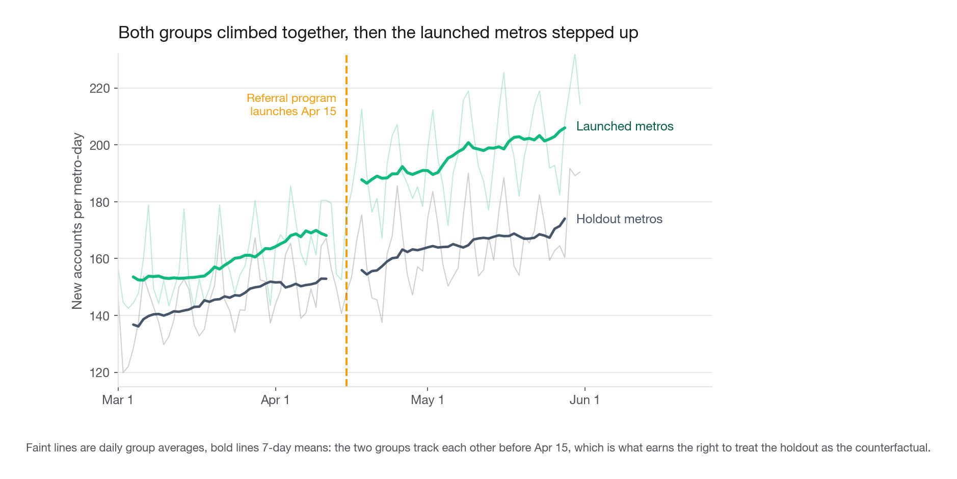
Step 4: The difference-in-differences estimate
Three specifications, in increasing order of how seriously you should take them.
The regression
Log signups per metro-day, metro fixed effects to absorb permanent size differences, date fixed effects to absorb everything that hits all eight metros on a given day, and the interaction you care about.
fit = smf.ols("ln ~ C(market) + C(first_date) + tr:post", data=panel.assign(
    post=panel.post.astype(int))).fit(cov_type="cluster", cov_kwds={"groups": panel.market})
b = fit.params["tr:post"]
lo, hi = fit.conf_int().loc["tr:post"]
print(round(100 * (np.exp(b) - 1), 1), round(100 * (np.exp(lo) - 1), 1), round(100 * (np.exp(hi) - 1), 1))
9.7 5.6 14.0The program lifted new account acquisition by 9.7 percent, with a 95 percent interval from 5.6 to 14.0 percent. Notice what happened to the headline: 23.5 percent became 9.7 percent, and roughly 60 percent of the apparent lift was the market growing on its own.
Eight clusters is not enough clusters
That interval is too narrow and you should say so unprompted. Cluster-robust standard errors are justified by an asymptotic argument in the number of clusters. With eight metros, that argument does not apply, and the resulting intervals are known to be too tight, sometimes badly. Do not report the number and hope nobody notices.
The honest small-sample move is to collapse the data to one observation per metro and run a plain two-sample t-test on four versus four.
w = panel.groupby(["market", "post"]).signups.mean().unstack()
w.columns = ["pre", "post"]
w["g"] = np.log(w.post) - np.log(w.pre)
from scipy import stats
a, c = w.loc[TREATED, "g"].values, w.drop(TREATED).g.values
se = np.sqrt(a.var(ddof=1) / 4 + c.var(ddof=1) / 4)
diff = a.mean() - c.mean()
print(round(100 * (np.exp(diff) - 1), 1), round(stats.ttest_ind(a, c).pvalue, 4),
      [round(100 * (np.exp(diff + s * 2.447 * se) - 1), 1) for s in (-1, 1)])
9.6 0.0031 [4.6, 14.8]Same point estimate, a wider interval, and six degrees of freedom you can defend to a statistician. This is the number to lead with.
Randomization inference closes the argument
There are exactly 70 ways to split eight metros into two groups of four. Compute the difference-in-differences for all 70 and see where the real assignment lands.
import itertools
ms = list(w.index)
obs = w.loc[TREATED, "g"].mean() - w.drop(TREATED).g.mean()
draws = np.array([w.loc[[ms[i] for i in c], "g"].mean()
                  - w.loc[[m for j, m in enumerate(ms) if j not in c], "g"].mean()
                  for c in itertools.combinations(range(8), 4)])
print(round(float((np.abs(draws) >= abs(obs)).mean()), 4))0.0286The observed split is the most extreme of the 70, in either direction. That gives p equal to 2 divided by 70, or 0.029, and here is the part worth internalizing: 0.029 is the smallest two-sided p-value this design can ever produce. Even an effect of 500 percent would return 0.029. Your evidence is capped by the number of metros, not by the size of the effect. Saying that in an interview signals you understand where inference actually comes from.
| Specification | Estimate | Interval | Why you would use it |
|---|---|---|---|
| Naive before-and-after | +23.5% | none | Never, except to show what it gets wrong |
| Two-way fixed effects, clustered | +9.7% | 5.6% to 14.0% | Point estimate and covariate adjustment |
| Metro-collapsed t-test | +9.6% | 4.6% to 14.8% | The interval you report |
| Randomization inference | +9.6% | p = 0.029, at the floor | The p-value you report |
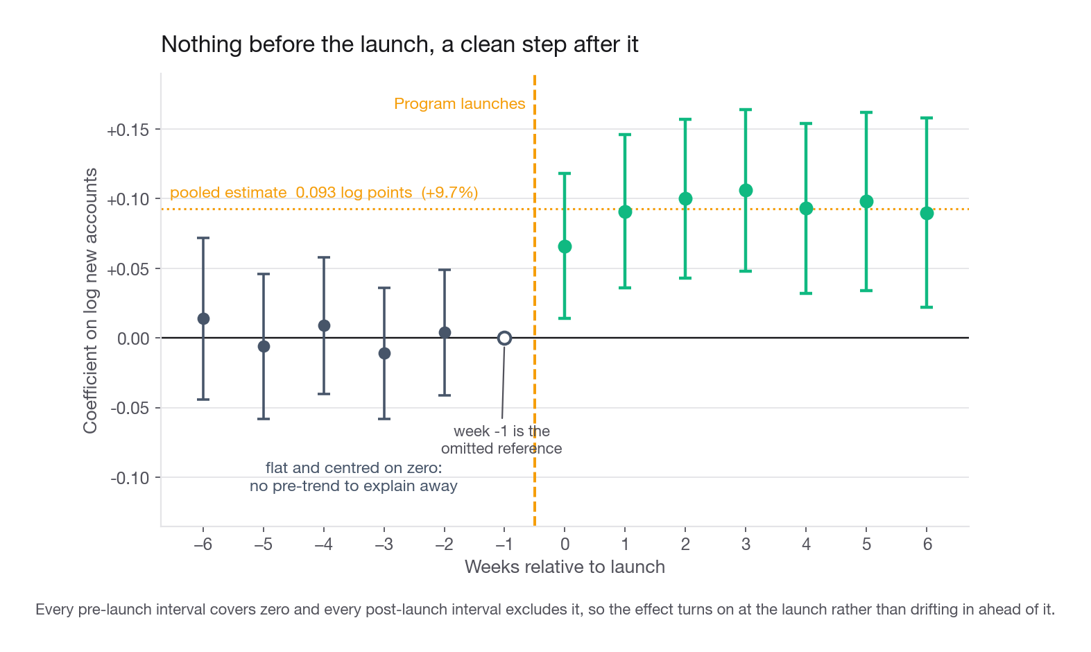
Interview tip: Report the metro-collapsed interval, not the clustered one, and explain in a sentence why. Interviewers who know the few-clusters literature will notice, and the ones who do not will still hear a candidate who knows why the two differ.
Step 5: Incremental, substituted, or manufactured
Now the part that separates the offer from the callback. Difference-in-differences told you the launched metros gained roughly a tenth more accounts than they otherwise would have. It said nothing about who those accounts are.
Attribution is not impact
Convert the percentage into people. The launched metros produced 36,971 new accounts in the 47 days after launch. Applying the holdout growth rate to their pre-launch level gives a counterfactual of 33,923. The difference is 3,048 accounts.
Meanwhile the referral attribution system claims credit for 16,934 accounts in the same window. Those two numbers describe the same event and differ by a factor of five and a half.
The gap is not a bug in either calculation. It is the entire finding. At most 18 percent of attributed referrals are additional accounts. The other 82 percent are accounts the market was going to produce anyway, which routed through a referral link because a link was there and it paid. Additional accounts, not additional people, and the decomposition is nested rather than a three-way split.
Manufactured accounts, and what the device tells you
The device_hash column looks like metadata. It is the most valuable column in the file. A referral program that pays the inviter creates a direct incentive to invite yourself: open a second account on the same phone, place one cheap order, collect 12 in credit.
acct["ref"] = (g.is_referred.mean() > 0.5).values & acct.launched & acct.post
acct["device"] = g.device_hash.first().values
shared = acct.groupby("device").size()
shared = set(shared[shared >= 2].index)
ref = acct[acct.ref]
base = acct[~acct.post].device.isin(shared).mean()
print(round(100 * ref.device.isin(shared).mean(), 1), round(100 * base, 1),
      int(ref.device.isin(shared).sum() - len(ref) * base))
30.8 5.0 4374Of the 16,934 attributed referrals, 30.8 percent sit on a device that already carries another Munch account. Among accounts created before the program existed, the same rate is 5.0 percent, which is your baseline for households sharing a tablet and for people who genuinely reinstall. The excess, roughly 4,374 accounts, is behaviour the program manufactured.
Now hold that against the lift. Difference-in-differences says the program created 3,048 accounts; the device evidence says 4,374 of the ones it paid for would not exist without it. The point estimates are incompatible, and subtracting leaves minus 1,326 genuinely new humans. Three readings survive and this data cannot separate them: the lift interval of 4.6 to 14.8 percent is 1,626 to 4,766 accounts and contains 4,374, so the floor is no real customers at all; or the lift sits near the top and a few hundred real people came with it; or 4,374 overstates, because a 5.0 percent baseline describes a world where nobody is paid 12 to invite a housemate. Say all three.
Do not stop at the count. Check whether the suspicious accounts behave differently, because a rate difference alone is circumstantial.
| Cohort | Accounts | Average basket | Revenue per account to 2026-05-31 | Placed a second order |
|---|---|---|---|---|
| New, not referred | 20,037 | 26.87 | 54.18 | 63.3% |
| New, referred, clean device | 11,718 | 21.84 | 34.92 | 45.3% |
| New, referred, shared device | 5,216 | 8.13 | about 8 | near zero |
| All new, referred | 16,934 | 18.84 | 26.67 | 31.4% |
Those are truncated observations, not lifetime values. Every account here was created between 2026-04-15 and 2026-05-31, so exposure runs 0 to 46 days and averages 22.5. The rows still compare cleanly because exposure is matched to within a quarter of a day, and revenue is front-loaded: pre-launch accounts with 60 or more days of history earn 86.6 percent of theirs in the first 22, so a full horizon lifts these figures by roughly 15 percent rather than multiplying them.
The shared-device group orders once, spends 8.13, and never returns. That is not a customer, it is a withdrawal. The clean referrals are real people who are simply worth about two thirds of an organic account. Both facts matter, and reporting only the blended 26.67 hides the more interesting half.
The cross-check hiding in revenue
Run the same difference-in-differences on daily order value instead of signups.
rp = orders.groupby(["market", "order_date"]).order_value.sum().rename("rev").reset_index()
rp["post"] = rp.order_date >= launch
r = rp.groupby(["market", "post"]).rev.mean().unstack()
r.columns = ["pre", "post"]
r["g"] = np.log(r.post) - np.log(r.pre)
gap = r.loc[TREATED, "g"].mean() - r.drop(TREATED).g.mean()
print(round(100 * (np.exp(gap) - 1), 1))-13.3Accounts up 9.6 percent, revenue down 13.3 percent, both against the same holdout, both with intervals that exclude zero. That combination looks contradictory until you do the arithmetic, and the arithmetic is what turns a contradiction into a mechanism.
Applying holdout revenue growth to the launched metros' pre-launch level gives a counterfactual of about 2,259,000 in the post window. Actual was 1,952,450, a shortfall of about 306,500. Split it two ways. The 3,048 incremental accounts added roughly 3,048 times 26.67, or about 81,300. The remaining attributed accounts, roughly 13,886 of them, were people who took a 26.67 path instead of a 54.18 path, costing about 13,886 times 27.51, or about 382,100. Those two terms sum to minus 300,800, which explains 98 percent of the observed shortfall.
Now be exact about what that buys you, because this is where candidates overclaim. Do not also invert the equation, report that it returns 2,940 against the signup estimate of 3,048, and call the two independent. It is one linear equation, so "explains 98 percent" and "agrees within four percent" are one number stated twice. Nor are the estimates independent: same accounts, same 47 days, same four metros against the same four holdouts, identical parallel-trends assumption. An unrelated April demand shock would inflate both and they would still agree. What it does rule out is a large arithmetic error and the wrong mechanism: for the implied count to halve, the revenue estimate would have to read about minus 17 percent rather than minus 13.3. That is a consistency check, not a second identification strategy.
Interview tip: When a second metric implies the same underlying number, say so, then immediately say what it does and does not rule out. Naming the assumption two checks share, before the interviewer names it, is worth more than the agreement itself, and candidates lose points for calling a consistency check triangulation.
Step 6: Does the program pay for itself
Everything so far is measurement. The recommendation needs a price.
Assume, and state, three numbers: contribution margin is 21 percent of order value after courier pay, restaurant share, and payment fees; 74 percent of issued credit is redeemed within 90 days; and each redeemed dollar costs Munch about 88 cents, because some credit lands on orders that would have happened anyway and some drives an extra order whose margin offsets part of the cost.
| Line | Value | How it is computed |
|---|---|---|
| Credits issued, face value | 203,208 | 16,934 payouts at 12 each |
| Effective credit cost | 132,329 | face value times 0.74 redemption times 0.88 |
| Incremental accounts | 3,048 | difference-in-differences on signups |
| Gross profit, ignoring the device evidence | 34,679 to 17,074 | 3,048 accounts at 54.18 or at the blended 26.67, 21 percent margin |
| Gross profit, netting out manufactured accounts | 4,464 or less | lift minus 4,374 at 54.18, taking the lift at the top of its interval |
| Return on spend | 0.26 to 0.13, or 0.03 and under after the device netting | gross profit divided by effective credit cost |
| Net, 47 days, four metros | minus 97,650 to minus 132,329 | gross profit minus effective credit cost |
On the first two bounds the program loses money at roughly four to eight times over, and neither bound is safe. The upper one assumes every incremental account behaves like an organic one, which the cohort table denies; both assume none of the lift was manufactured, which the device work makes unlikely. The third row is the only line surviving both, and even at the top of the lift interval it leaves 392 accounts worth about 4,464 against 132,329 of credit cost. One horizon caveat: those per-account values cover about 22 days while the credit clock runs 90, so a full horizon moves return on spend to about 0.30 and 0.15 and break-even credit to 3.63. The verdict does not turn on it.
Two candidate fixes, and the arithmetic matters more than the intuition.
The obvious one is anti-fraud. Block second accounts on a device that already has one and you remove about 4,374 payouts, cutting effective cost from 132,329 to about 98,150. Return on spend improves from 0.26 to 0.35 on the generous bound and from 0.13 to 0.17 on the conservative one. Still underwater either way, and note what the arithmetic assumes: it holds the 3,048 incremental accounts fixed while deleting 4,374 payouts from the denominator, which is only valid if none of the blocked accounts sits inside the lift. This is the answer most candidates give, and by itself it does not save the program, because manufactured accounts are only a quarter of the payouts. The rest is substitution, which no fraud rule can touch.
The lever that actually moves the number is when you pay. Pay the inviter only after the invited account places a second order and payouts drop from 16,934 to 5,321, because 68.6 percent of referred accounts never place one. Effective cost falls to about 41,580 and return on spend rises to 0.41 on the conservative bound and 0.83 on the generous one. That is 1.2 to 2.4 times underwater instead of four to eight, which is the difference between a redesign worth piloting and a shutdown, but only if referred accounts sit closer to the organic end, and that is a measurable question rather than an assumption you get to make.
Two things it does not do. It does not remove manufactured accounts for free: ordering once is a response to a payout that triggers on the first order, not a property of those accounts, and a self-referrer facing a second-order trigger places one more 8.13 order to unlock a 12 credit, buying Munch 1.71 of margin. Pair the trigger change with the device block rather than treating it as a substitute. And it reprices the observed program under a new rule instead of forecasting the redesigned one, holding volume and the 31.4 percent second-order rate at values the old rule produced. If volume falls, numerator and denominator fall together and the ratio barely moves; if inviters coach a second order to collect, payouts rise against an unchanged incremental count and 0.83 falls. Both elasticities belong in the follow-up test.
For completeness, solve for the credit that breaks even at the current design: 1.55 to 3.14, against the 12 being paid. Nobody refers a friend for 3.14, and certainly not for 1.55. That is the clearest possible statement that the problem is structural, not a matter of tuning the payout.
One framing point, because it decides which line you attack. In revenue terms substitution is the biggest number, 382,100 against 132,329 of credits. Apply the 21 percent margin and it inverts: substitution costs about 80,200 of contribution, the credits 132,329 in cash. On the basis Munch banks, credits are the largest single line, which is why the payout trigger is the fix.
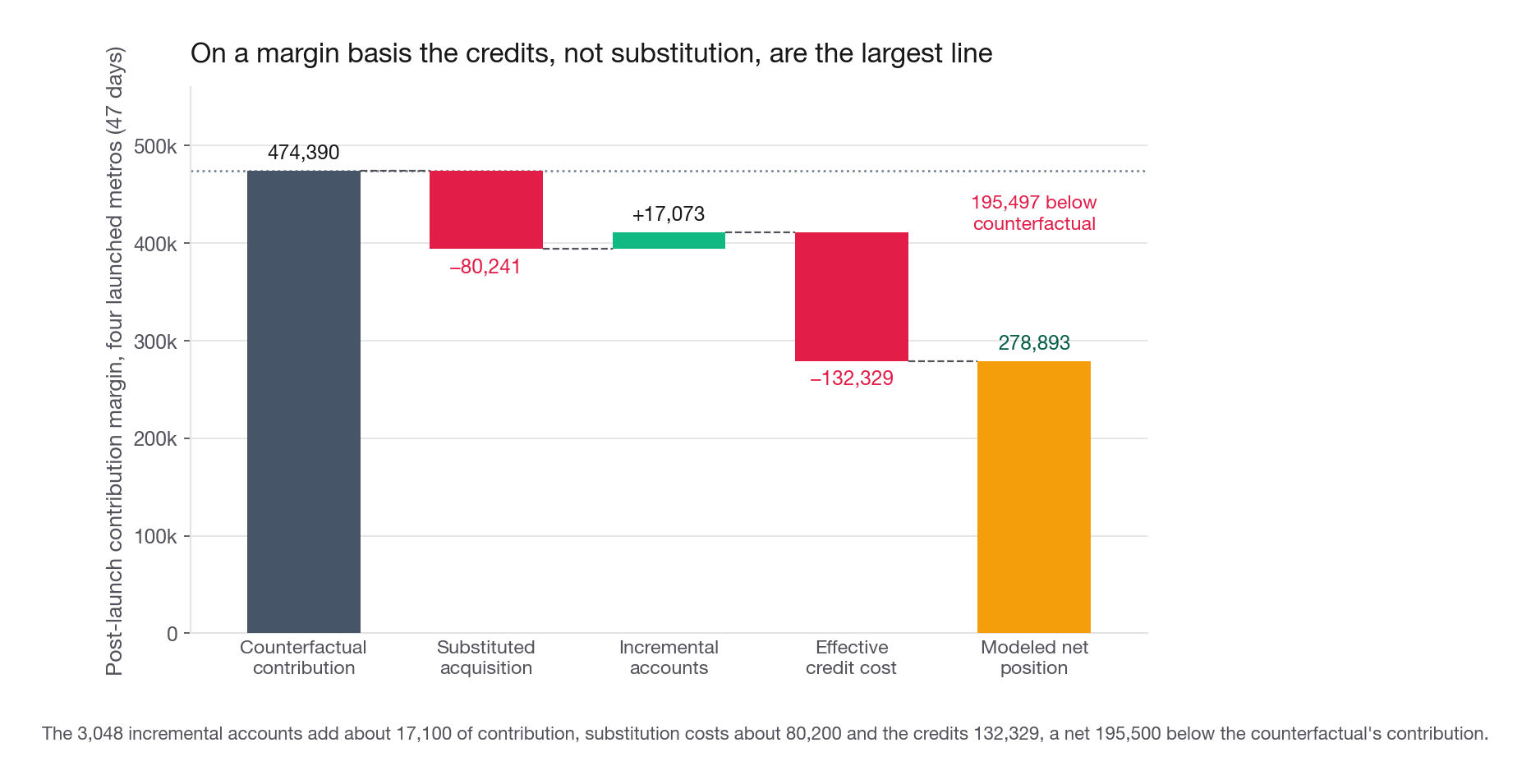
Step 7: The experiment you should have run
The last question on this challenge is always some version of "how would you test this properly", and it has a specific right answer.
You cannot randomize individual users. A referral program is a message from one person to another, so treating Ana and holding out Ben does not work: Ana invites Ben, Ben signs up, and Ben's outcome now depends on Ana's assignment. That violates the no-interference assumption that user-level randomization rests on, and it contaminates the control arm in exactly the direction that makes the program look worse than it is. Say this before you propose anything, because it is the reason the obvious design is unavailable.
For a geo test, power is the whole conversation, and the unit is the metro. The between-metro standard deviation of log growth in this data is 0.027. That gives the following minimum detectable effects at 80 percent power and a 5 percent two-sided test.
| Metros per arm | Degrees of freedom | Minimum detectable lift |
|---|---|---|
| 4 | 6 | 6.6% |
| 6 | 10 | 5.0% |
| 8 | 14 | 4.1% |
| 10 | 18 | 3.6% |
| 20 | 38 | 2.5% |
The design Munch stumbled into could only detect a lift of 6.6 percent or larger. The true effect was 9.6 percent, so it got lucky. If the program had delivered a perfectly respectable 4 percent lift, this exact analysis would have returned nothing, and somebody would have concluded the program does not work. Explaining that distinction, between a null result and an underpowered one, is the single most useful thing you can say about experimental design.
Practical recommendation for the next round: keep the four holdout metros dark for another eight weeks and open four new ones randomized into the holdout arm, giving six per arm across twelve metros and a 5.0 percent minimum detectable lift instead of 6.6, noting that a 4 percent lift stays underpowered at about 62 percent because eight per arm means sixteen metros Munch does not operate; pay the inviter only on the invited account's second order; block second accounts per device at signup and log the block rather than silently dropping it, so the block rate is measurable; and instrument the invited account's metro at signup rather than inferring it from orders, so cross-metro spillover becomes countable instead of assumed away.
Step 8: Writing it up
The submission is graded on whether the decision maker can act on it, not on how much you did.
One thing to resist. You will be tempted to lead with the negative revenue difference-in-differences because it is dramatic. Do not. Lead with the incrementality number, because that is what the decision hinges on, and bring the revenue result in as corroboration. A finding that contradicts a manager's expectation lands better when it arrives as the second piece of evidence rather than the first.
Common traps
Reporting the before-and-after change as the impact. It bundles seasonality, secular growth, and every other thing that shipped that week. Fix: always compute the same change for an untreated group and report both.
Treating attributed referrals as incremental users. Attribution answers "which path did this person take", not "would this person exist otherwise". Fix: estimate incrementality from a comparison group and treat the attribution count as an upper bound.
Announcing that parallel trends holds because a test returned p above 0.05. With eight units the test barely has power to detect anything. Fix: report the estimated pre-trend, its sign, and what size of pre-trend you would have detected.
Reporting cluster-robust intervals with eight clusters. The justification is asymptotic in the cluster count and does not apply. Fix: collapse to one observation per unit and use a t-test, or use randomization inference, and say why.
Fixing the referral flag silently. Two percent of accounts carry both values, and your rule changes the denominator of every rate. Fix: state the rule, state the alternative, report how much the answer moves.
Ignoring device identifiers. They are the only column that can detect self-referral, which was 30.8 percent of payouts against a 5.0 percent baseline. Fix: check identifier reuse against a pre-period baseline before calling anything fraud.
Proposing user-level randomization for a social feature. Treated users invite control users, so the arms contaminate each other. Fix: randomize at the level that contains the spillover, usually the metro, and accept the power cost explicitly.
Recommending a fraud crackdown as the fix. Manufactured accounts were 4,374 of 16,934 payouts. Removing all of them still leaves the program underwater. Fix: price each remedy separately before recommending it.
Quoting a p-value below the design's floor. With four metros per arm, randomization inference cannot return anything under 0.029. Fix: know the floor of your own test before you report a number below it.
Stopping once the model runs. The regression is 20 minutes of the work. The decomposition, the pricing, and the redesign are what get scored.
Quick self-check
Answer these out loud, in full sentences, before you look anything up.
The launched metros grew 23.5 percent and the holdout metros grew 13.5 percent over the same window. Explain in one sentence why 9.6 percent, and not 23.5 percent, is the causal estimate, and name the specific thing the holdout absorbs.
Your pre-trend test returns a coefficient of minus 0.00102 per day with a p-value of 0.259. State what that does and does not license you to claim, and say which direction it biases the headline if it is real.
Distinguish an attributed account that is not incremental from one that is incremental but worthless. Name the column in this file that identifies the second kind, and say why only the first can be read straight off the attribution table.
Signups rose 9.6 percent against the holdout while revenue fell 13.3 percent against the same holdout. Reconcile the two with arithmetic, not adjectives.
Blocking duplicate devices removes 4,374 of 16,934 payouts and moves return on spend from 0.26 to 0.35, or 0.13 to 0.17 on the conservative bound. Explain why that is not enough, give the range the payout-trigger change reaches, and name what both scenarios hold fixed that the change would itself move.
You have 20 comparable metros and 10 weeks. Design the follow-up test: the unit of randomization, the arms, the primary metric, the minimum detectable effect, and the one thing you would refuse to change mid-test.
If question 4 gave you trouble, go back and write the two-term decomposition on paper. It is the piece that converts a competent analysis into one a manager can act on.