5.1 Challenge: Analyzing a Pricing Test
Find the core decision, design, or behavior signal.
Turn the lesson into a concise response blueprint.
Name the trap you would avoid in a real interview.
Use these checkpoints as your reading path before diving into the full lesson.
- 1Why this matters in interviews
- 2The brief you were handed
- 3Build the table before you build the op...
- 4Trust checks that come before any p-value
- 5The price column that argues with the a...
Gridline sells a project-tracking tool to small engineering teams at 49 per seat per month. Growth has stalled, the head of product wants to know whether 79 would print more money, and for six weeks a third of arriving visitors have been shown the higher price. You have been handed the assignment log and asked one question that sounds simple and is not: which price should we ship? This lesson walks the whole path from raw assignment rows to a recommendation you can defend when the room pushes back, including the part most candidates skip, which is deciding what you would have needed to see in order to say no.
Why this matters in interviews
Pricing tests are the most common experimentation take-home for a reason. They compress almost every skill an experimentation interviewer wants to probe into one dataset: metric selection under a mechanical tradeoff, a heavy-tailed outcome variable that breaks naive tests, an assignment log that has to be validated before it can be trusted, segment effects that are real and segment effects that are noise, and a stopping-rule question that separates people who have run experiments from people who have read about them.
The trap is that the arithmetic is easy. Conversion rate, revenue per visitor, a two-sample test, done in twenty minutes. Candidates who stop there get dinged for not interrogating the data or for a recommendation that is not decision-ready. The gap is not statistical sophistication. A price change is not a feature launch: raising price mechanically trades volume for margin, so a revenue-neutral result is a strategic shift disguised as a null. Surface that trade and put a number on both sides of it.
Interviewers also like this problem because the counterfactual is legible to non-technical stakeholders. A VP can argue with your churn model. Nobody argues with "at 79 we sign 61 fewer teams a day."
Interview tip: Open your write-up with the decision and the tradeoff in two sentences, then show the work. Graders read the top of the document with full attention and skim the middle.
The brief you were handed
Two tables. The first is the assignment log, one row per visitor who reached the pricing page for the first time. The second is a lookup of account metadata that joins on the visitor key. The design was a 65/35 split favouring the incumbent price, which is the standard risk-averse choice when the treatment could plausibly cost real revenue.
| Column | Table | Meaning | Watch out for |
|---|---|---|---|
visitor_id | both | first-touch visitor key | duplicates mean re-randomisation |
assigned_at | assignment log | timestamp of first pricing-page view | local time versus UTC |
variant | assignment log | control or treatment | the design intent, not what shipped |
price_shown | assignment log | 49 or 79 | must agree with variant |
channel | assignment log | acquisition source | pre-assignment, safe to segment on |
device | assignment log | desktop or mobile | pre-assignment, safe to segment on |
converted | assignment log | bought a plan in the window | post-assignment |
seats | assignment log | seats on the purchased plan | post-assignment, heavy right tail |
The three questions on the brief are: should Gridline ship 49 or 79, what did you learn about how different users respond, and did the test need to run for six weeks or could it have been called earlier.
The last one is phrased as a bonus. Treat it as the main event: it reveals whether you understand power, and it is where most candidates confidently give the wrong answer.
Build the table before you build the opinion
Everything below runs on this generator. It produces the exact schema described above, with the same seed, so every number quoted in this lesson is reproducible on your machine.
import numpy as np
import pandas as pd

SEED = 20261
rng = np.random.default_rng(SEED)
N = 240_000

channels = np.array(["paid_search", "paid_social", "organic_search",
                     "partner_referral", "direct"])
channel = rng.choice(channels, size=N, p=[0.31, 0.19, 0.22, 0.11, 0.17])
device = rng.choice(["desktop", "mobile"], size=N, p=[0.63, 0.37])
variant = rng.choice(["control", "treatment"], size=N, p=[0.65, 0.35])
price_shown = np.where(variant == "treatment", 79, 49)
day = rng.integers(0, 42, size=N)

pull = pd.Series({"paid_search": 0.0, "paid_social": -0.38, "organic_search": 0.26,
                  "partner_referral": 0.64, "direct": 0.33}).reindex(channel).to_numpy()
logit = (-3.45 + pull + 0.20 * (device == "desktop")
         - 0.42 * (variant == "treatment")
         + 0.30 * ((variant == "treatment") & (device == "mobile")))
converted = rng.binomial(1, 1 / (1 + np.exp(-logit)))
seats = converted * (1 + rng.poisson(np.where(variant == "treatment", 2.15, 2.5), size=N))

pt = pd.DataFrame({"visitor_id": np.arange(700_000, 700_000 + N),
                   "assigned_at": pd.Timestamp("2026-03-02") + pd.to_timedelta(day, unit="D"),
                   "variant": variant, "price_shown": price_shown, "channel": channel,
                   "device": device, "converted": converted, "seats": seats})
swapped = rng.random(N) < 0.0009
pt.loc[swapped, "price_shown"] = np.where(pt.loc[swapped, "variant"] == "control", 79, 49)
broken = (day == 11) & (variant == "treatment") & (rng.random(N) < 0.55)
pt.loc[broken, ["converted", "seats"]] = 0
pt["revenue"] = pt["converted"] * pt["price_shown"] * pt["seats"]
That gives 240,000 assignment rows spanning 2026-03-02 through 2026-04-12, which is 42 calendar days at roughly 5,700 visitors per day. Revenue per visitor is defined as price times seats for buyers and zero for everyone else, which is first-month billed revenue, not lifetime value. Say that out loud in the write-up. It matters later.
Trust checks that come before any p-value
Four checks, in this order, before you compute a single treatment effect. Each one has a specific failure mode and a specific response, and interviewers notice when you run them in the wrong order or skip straight to the test.
The price column that argues with the assignment flag
The log carries both variant and price_shown. Two columns encoding the same fact is an invitation. Cross-tabulate them.
print(pd.crosstab(pt["variant"], pt["price_shown"]))

mismatch = (((pt["variant"] == "control") & (pt["price_shown"] == 79))
            | ((pt["variant"] == "treatment") & (pt["price_shown"] == 49)))
print(mismatch.sum(), round(100 * mismatch.mean(), 3))

exp = pt.loc[~mismatch].copy()
price_shown 49 79
variant
control 155512 156
treatment 82 84250
238 0.099238 rows, about one in a thousand, were served a price that contradicts their bucket. What you do with them is a question about which estimand you report, not about cleaning. The default headline is intent to treat: analyse every assigned row by the bucket the randomiser wrote, whatever the page rendered. Dropping them, which is what exp above does, is a per-protocol analysis conditioned on price_shown, a column written after randomisation. That is the same move this lesson warns about elsewhere, so it belongs beside the headline as a sensitivity check, not in front of it.
Leakage attenuates the intent-to-treat estimate roughly in proportion to the crossover rate, here one row in a thousand, which is why the assignment-based and delivered-price estimates below differ by 0.003 points. When crossover is material the remedy is a complier-average or instrumental-variables estimate reported next to intent to treat, never deletion. Keeping the rows silently is wrong. Keeping them as your primary estimate and showing the exclusion alongside is right, and it is the answer you need when an interviewer asks whether excluding on a post-randomisation column breaks your randomisation. Escalate them to engineering regardless, on engineering grounds: a path leaking one assignment in a thousand may be leaking something larger elsewhere.
Interview tip: When two columns are supposed to encode the same fact, cross-tabulate them within the first ten minutes. A challenge that ships both columns is usually testing whether you check.
Sample ratio mismatch
The design said 65/35. Test it rather than eyeballing it.
from scipy import stats

n = exp["variant"].value_counts()
expected = [len(exp) * 0.65, len(exp) * 0.35]
chi2, p = stats.chisquare([n["control"], n["treatment"]], f_exp=expected)
print(n.to_dict(), round(chi2, 2), round(p, 3))
{'control': 155512, 'treatment': 84250} 2.04 0.154Chi-square 2.04, p equal to 0.154. The split is consistent with the design. Report this in one line, because if it had failed the entire analysis would be dead. A sample ratio mismatch means the randomiser or the logger dropped users non-randomly, and no amount of downstream statistics repairs that. The correct response to a failed SRM is not a covariate adjustment, it is to stop and find the leak.
Be ready for the follow-up: what counts as a fail? Use p below 0.001, because SRM tests run on huge samples and the alarm should mean something. A p of 0.03 on two million rows is a rounding artifact.
Balance on pre-assignment attributes
Randomisation should have distributed channel and device identically across arms. Check the two variables you plan to segment on, because if they are imbalanced then every segment comparison you make later inherits that imbalance.
for col in ["channel", "device"]:
    tab = pd.crosstab(exp[col], exp["variant"])
    chi2, p, _, _ = stats.chi2_contingency(tab)
    print(col, round(chi2, 2), round(p, 3))
    print(((tab / tab.sum()) * 100).round(2))
Channel gives chi-square 7.40 with p equal to 0.116 across five categories, device gives 0.21 with p equal to 0.646. Paid search sits at 31.1 percent of control and 30.8 percent of treatment, mobile at 36.9 versus 37.0. Nothing to see, which is exactly what you want to be able to say.
Only test variables fixed before assignment. Testing balance on converted or seats is not a balance check, it is the treatment effect, and candidates do confuse the two.
The day the treatment pricing page broke
Now plot the daily series per arm. This single step catches more real problems than every other check combined.
exp["day"] = (exp["assigned_at"] - exp["assigned_at"].min()).dt.days
daily = exp.pivot_table(index="day", columns="variant",
                        values="converted", aggfunc="mean") * 100
baseline = daily["treatment"].drop(11).mean()
print(round(baseline, 2))
print(daily[daily["treatment"] < 0.5 * baseline].round(2))
3.03
variant control treatment
day
11 4.40 0.97On 2026-03-13, a Friday, treatment conversion fell to 0.97 percent against a run-rate of 3.03 percent, while control held at 4.40 percent. Nineteen purchases where roughly 59 were expected from 1,956 visitors, which is more than five standard errors below trend. Control was fine that day, so this is not a traffic story or a holiday, it is the treatment pricing page failing for part of a day.
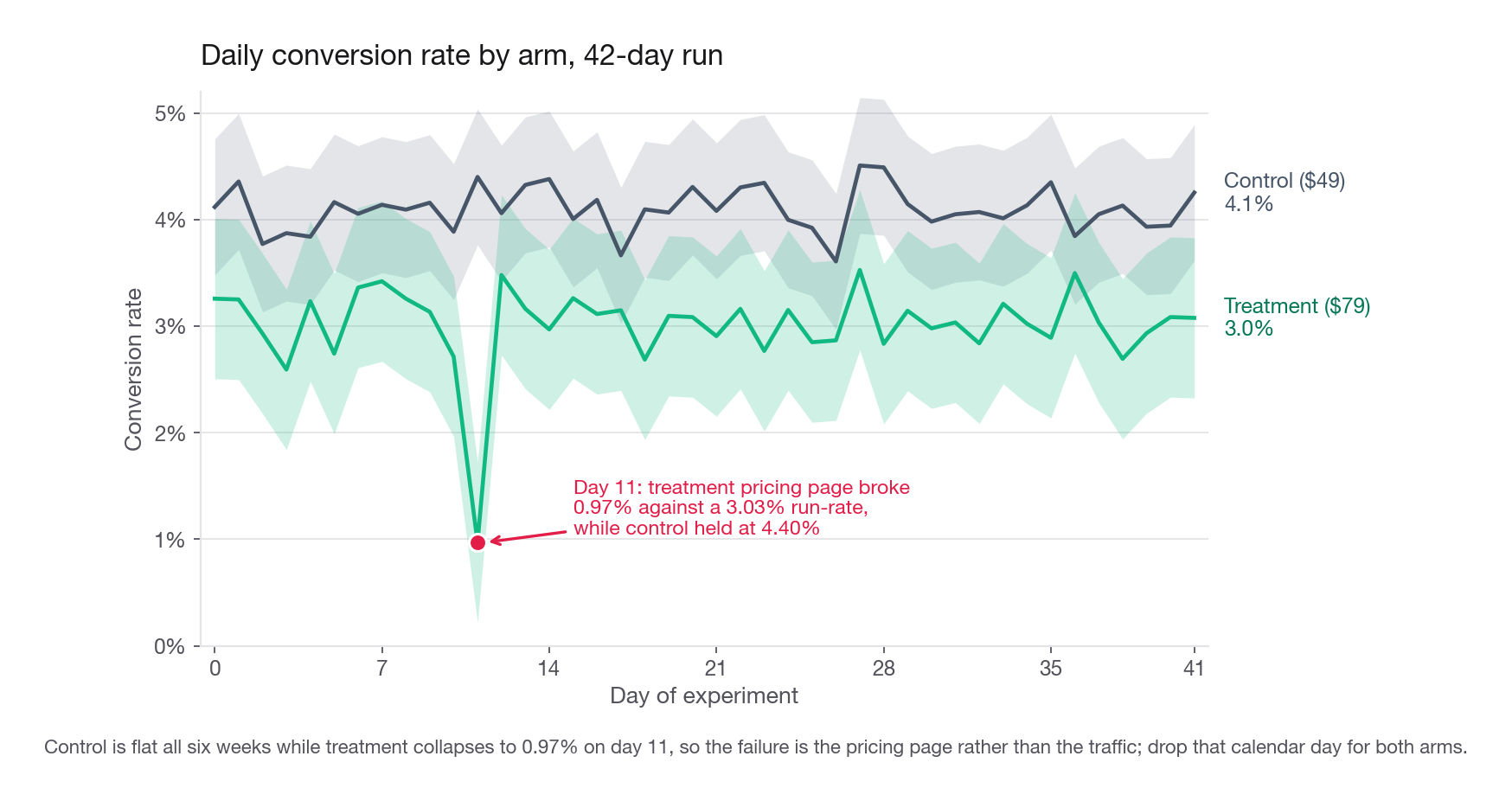
Drop the day. Not the arm, not the users, the whole calendar day for both arms, so that the comparison stays balanced on whatever else was happening that Friday.
clean = exp[exp["day"] != 11].copy()
summary = clean.groupby("variant").agg(
    visitors=("visitor_id", "size"),
    conv_rate=("converted", "mean"),
    arpv=("revenue", "mean"))
summary["aov"] = summary["arpv"] / summary["conv_rate"]
print(summary.round(4))
visitors conv_rate arpv aov
variant
control 151735 0.0410 7.0703 172.5878
treatment 82294 0.0303 7.5550 249.5905234,029 rows survive. Note how much this one exclusion matters: leaving the broken Friday in gives a treatment revenue lift of 4.90 percent with p equal to 0.065, and removing it gives 6.86 percent with p equal to 0.0115. The difference between "no effect detected" and "significant effect" was a single corrupted day out of 42.
Interview tip: Always report the headline number both with and without any exclusion you make. If the conclusion flips, that fragility is itself a finding and hiding it is what gets candidates rejected.
Name the estimand before you name the number
That rule applies to the 238 mismatched rows too, and honouring it costs three extra numbers.
pt["day"] = (pt["assigned_at"] - pt["assigned_at"].min()).dt.days
itt = pt[pt["day"] != 11]

def lift(df, col, hi):
    x = df.loc[df[col] == hi, "revenue"].to_numpy()
    y = df.loc[df[col] != hi, "revenue"].to_numpy()
    d = x.mean() - y.mean()
    s = np.sqrt(x.var(ddof=1) / len(x) + y.var(ddof=1) / len(y))
    return f"{100 * d / y.mean():.2f}  {2 * (1 - stats.norm.cdf(abs(d / s))):.4f}"

print("intent to treat ", len(itt), lift(itt, "variant", "treatment"))
print("as treated      ", len(itt), lift(itt, "price_shown", 79))
print("per protocol    ", len(clean), lift(clean, "variant", "treatment"))
intent to treat 234256 6.82 0.0119
as treated 234256 6.82 0.0118
per protocol 234029 6.86 0.0115The three agree to 0.04 points, so nothing here turns on the choice. Say that out loud, then say why intent to treat is still primary: it does not require assuming the leak was independent of who was going to buy. It probably was, but no column in this log lets you check. The rest of this lesson quotes the per-protocol frame clean, and every headline should carry the intent-to-treat figure beside it.
Choosing the metric you will actually decide on
Conversion rate is the wrong headline for a pricing test, and saying so early is worth points. Raising the price will lower conversion. That is not a finding, it is arithmetic. The only interesting question is whether the higher take per buyer more than pays for the lost buyers.
| Metric | What it measures | Why it is the wrong headline here | Keep it because |
|---|---|---|---|
| Conversion rate | share of visitors who buy | falls by construction when price rises | it is precise and diagnoses where the loss lands |
| Average order value | revenue per buyer | rises by construction, and is conditioned on a post-treatment event | it separates the price effect from the seat effect |
| Seats per account | plan size chosen | selection: only buyers appear | it localises where the order-value rise comes from |
| Revenue per visitor | the whole tradeoff in one number | nothing, this is the decision metric | it prices volume and margin on the same scale |
Revenue per visitor is the decision metric because it is defined on every randomised unit and therefore inherits the randomisation. Average order value is not: it is computed only over buyers, and the set of buyers is different in each arm. If price rises and the marginal buyer who drops out was a small team, average order value climbs partly because the low end was censored, not because anyone bought more. That is a textbook post-treatment conditioning bias, and interviewers ask about it directly.
The three headline moves in this test:
| Quantity | 49 per seat | 79 per seat | Relative change |
|---|---|---|---|
| Conversion rate | 4.10% | 3.03% | -26.1% |
| Seats per purchased plan | 3.53 | 3.16 | -10.3% |
| Revenue per visitor | 7.07 | 7.56 | +6.9% |
Three effects stack: 61 percent more list price, 26 percent fewer buyers, and 10 percent fewer seats among the buyers who remain. Multiply them out, 1.612 times 0.739 times 0.897, and you land near 1.07. That is exact accounting for the revenue-per-visitor ratio, and showing it is worth points on its own.
The seat term is the one candidates want to read behaviourally, and that is where the trap sits. Seats per buyer conditions on the same post-treatment event as average order value, which is only 79/49 times it, so the minus 10 percent mixes real downsizing with a shift in who still buys. Composition runs the same direction: at 79 per seat a ten-person team faces a 790 monthly bill, so larger teams are the likelier dropouts and seats per buyer falls with nobody touching their roster. The quantity you can defend is seats per visitor, defined on every assigned unit, 0.144 in control against 0.096 in treatment, down 33.7 percent.
Roster trimming is therefore a hypothesis, not a finding, and this log cannot settle it: seats is zero for every non-buyer, so team size is unobserved for precisely the visitors who walked away. Settling it needs a pre-assignment covariate the log does not carry, company size at signup or the seat count chosen before checkout. The seat-selection change waits on that, and saying so is stronger than asserting the behavioural reading.
Running the test properly
The outcome variable is 96 percent zeros
Revenue per visitor here has a pooled standard deviation of 42.88 against a mean of 7.07, so the coefficient of variation is about 6.1. Roughly 96 percent of rows are exactly zero and the non-zero tail runs from 49 up to 869. Skewness is about 6 in control and 7 in treatment.
None of that invalidates a t-test. The central limit theorem is operating on group means of 82,000 and 152,000 observations, and at that size the sampling distribution of the mean is essentially normal even for an outcome this lumpy. What the skew does do is inflate the standard error, which is why the conversion comparison is decisive at p near 1e-39 while the revenue comparison sits at p near 0.01 on the same data.
Use Welch rather than the pooled-variance version, because the arms genuinely have different variances: the treatment arm's non-zero values are all at least 79, so its spread is wider.
a = clean.loc[clean["variant"] == "treatment", "revenue"].to_numpy()
b = clean.loc[clean["variant"] == "control", "revenue"].to_numpy()
diff = a.mean() - b.mean()
se = np.sqrt(a.var(ddof=1) / len(a) + b.var(ddof=1) / len(b))
lo, hi = diff - 1.96 * se, diff + 1.96 * se
print(round(diff, 4), round(se, 4), (round(lo, 3), round(hi, 3)))
print([round(100 * x / b.mean(), 2) for x in (diff, lo, hi)])
0.4847 0.1918 (0.109, 0.861)
[6.86, 1.54, 12.17]An absolute gain of 0.49 per visitor, 95 percent interval from 0.11 to 0.86, which is plus 6.86 percent relative with an interval from plus 1.5 percent to plus 12.2 percent. Quote the interval, not the point estimate. "Somewhere between one and a half and twelve percent" is the honest summary, and the width of that band is the thing the rest of the lesson is about.
Confirm with a bootstrap, because it costs nothing
boot = np.random.default_rng(7)
ratios = np.empty(2000)
for i in range(2000):
    ia = boot.integers(0, len(a), len(a))
    ib = boot.integers(0, len(b), len(b))
    ratios[i] = a[ia].mean() / b[ib].mean()
print(round(100 * (ratios.mean() - 1), 2),
      np.round(100 * (np.quantile(ratios, [0.025, 0.975]) - 1), 2))
6.89 [ 1.55 12.3 ]The percentile bootstrap gives plus 6.89 percent with an interval from 1.55 to 12.30. It agrees with Welch to two decimal places, which tells you the normal approximation is fine at this sample size. Run it anyway, because a two-line bootstrap is the cheapest way to pre-empt "but the distribution is not normal" from a sceptical interviewer.
Winsorize seats, never dollars
The standard robustness check on a skewed revenue metric is to cap the tail. Here that check will mislead you if you do it the obvious way. Capping revenue at 395 per visitor halves the effect and kills the significance, as if most of it were a handful of whales.
dollar = clean["revenue"].clip(upper=395)
x = dollar[clean["variant"] == "treatment"].to_numpy()
y = dollar[clean["variant"] == "control"].to_numpy()
d = x.mean() - y.mean()
s = np.sqrt(x.var(ddof=1) / len(x) + y.var(ddof=1) / len(y))
print(round(100 * d / y.mean(), 2), round(2 * (1 - stats.norm.cdf(abs(d / s))), 4))
3.57 0.1715Plus 3.57 percent at p equal to 0.17, down from plus 6.86 at p equal to 0.0115.
It is an artifact. A fixed dollar cap censors the two arms at different seat counts, because the arms have different prices. 49 times 8 is 392, which fits under the cap, so control is capped above 8 seats. 79 times 5 is 395, exactly the cap, so treatment is capped above 5 seats. You have quietly truncated the treatment arm three seats earlier than control, which mechanically removes treatment revenue. Cap the unit of behaviour instead.
for cap in [8, 10, 12]:
    capped = clean["converted"] * clean["price_shown"] * clean["seats"].clip(upper=cap)
    x = capped[clean["variant"] == "treatment"].to_numpy()
    y = capped[clean["variant"] == "control"].to_numpy()
    d = x.mean() - y.mean()
    s = np.sqrt(x.var(ddof=1) / len(x) + y.var(ddof=1) / len(y))
    print(cap, round(100 * d / y.mean(), 2),
          round(2 * (1 - stats.norm.cdf(abs(d / s))), 4))
8 7.05 0.0093
10 6.87 0.0113
12 6.86 0.0114Capping at 8 seats, which touches only 43 of 234,029 rows, leaves the effect at plus 7.05 percent. The result is not a tail artifact. Say that explicitly, because "I checked the obvious fragility and it held" is a stronger sentence than never mentioning fragility at all.
Interview tip: Any transformation applied to a monetary outcome must be applied in units both arms share. When arms differ in price, cap quantity, cap percentiles computed within arm, or do not cap at all.
Segmentation without p-hacking
You have two pre-assignment attributes to slice on, which means two families of subgroup tests. With five channels and two devices you are running seven comparisons, and at alpha 0.05 you expect roughly one false positive by chance alone. Discipline here is what separates a segmentation section that adds credibility from one that destroys it.
def segment_lift(df, col):
    rows = []
    for key, g in df.groupby(col):
        x = g.loc[g["variant"] == "treatment", "revenue"].to_numpy()
        y = g.loc[g["variant"] == "control", "revenue"].to_numpy()
        d = x.mean() - y.mean()
        s = np.sqrt(x.var(ddof=1) / len(x) + y.var(ddof=1) / len(y))
        rows.append({col: key, "n": len(g),
                     "lift_pct": 100 * d / y.mean(),
                     "lo": 100 * (d - 1.96 * s) / y.mean(),
                     "hi": 100 * (d + 1.96 * s) / y.mean(),
                     "p": 2 * (1 - stats.norm.cdf(abs(d / s)))})
    return pd.DataFrame(rows).sort_values("n", ascending=False)
Channel: one interesting result that does not survive correction
| Channel | Visitors | Conversion change | Revenue per visitor lift | 95% interval | p |
|---|---|---|---|---|---|
| paid_search | 72,635 | -28.5% | +6.4% | -4.1% to +17.0% | 0.233 |
| organic_search | 51,521 | -29.9% | -0.1% | -10.4% to +10.1% | 0.978 |
| paid_social | 44,512 | -27.9% | +7.6% | -8.3% to +23.6% | 0.347 |
| direct | 39,735 | -22.7% | +8.2% | -3.5% to +19.8% | 0.168 |
| partner_referral | 25,626 | -19.5% | +16.3% | +3.0% to +29.6% | 0.016 |
Partner referral looks like the star: the smallest conversion loss and the largest revenue gain. It is also the only one of five with p below 0.05, and 0.05 divided by 5 is 0.01, so it does not clear a Bonferroni bar. Fit the interaction directly rather than arguing from a table of five p-values, and the interaction term lands at p equal to 0.062. Suggestive, not established.
The right sentence is: referral traffic appears least price-sensitive, consistent with the story that a warm introduction from an existing team raises willingness to pay, but with 25,600 visitors this run cannot separate that from noise, and I would want a dedicated follow-up before pricing on it.
Device: an interaction that is real
| Device | Visitors | Conversion change | Revenue per visitor | Lift | 95% interval | p |
|---|---|---|---|---|---|---|
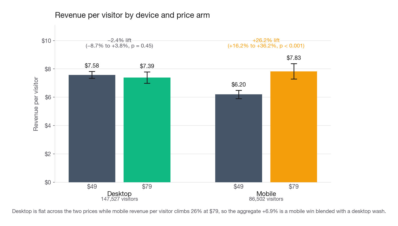
| desktop | 147,527 | -31.7% | 7.58 to 7.39 | -2.4% | -8.7% to +3.8% | 0.447 |
| mobile | 86,502 | -14.5% | 6.20 to 7.83 | +26.2% | +16.2% to +36.2% | 0.000 |
This one is not marginal. Mobile visitors barely reduce their conversion when price rises, 14.5 percent against desktop's 31.7 percent, and their revenue per visitor climbs 26 percent with an interval nowhere near zero. Desktop is flat to slightly negative. The aggregate plus 6.9 percent is a blend of a large mobile win and a desktop wash.
Do not stop at two subgroup tests. Fit the interaction, which is the test of whether the difference between the two lifts is itself distinguishable from noise.
import statsmodels.formula.api as smf

clean["T"] = (clean["variant"] == "treatment").astype(int)
clean["mob"] = (clean["device"] == "mobile").astype(int)
fit = smf.ols("revenue ~ T * mob", data=clean).fit(cov_type="HC1")
print(fit.summary2().tables[1].round(3))
Coef. Std.Err. z P>|z| [0.025 0.975]
Intercept 7.577 0.126 59.957 0.000 7.330 7.825
T -0.184 0.242 -0.761 0.447 -0.657 0.290
mob -1.374 0.195 -7.027 0.000 -1.757 -0.990
T:mob 1.809 0.397 4.556 0.000 1.031 2.588The interaction coefficient is 1.81 with z equal to 4.56. Heteroskedasticity-robust errors, because the arms have unequal variance. This is the single most quotable result in the analysis: the price effect on mobile is 1.81 higher per visitor than on desktop, and that gap is nailed down.
Before building a strategy on it, ask what mobile is proxying for. At Gridline, mobile skews toward founders and team leads browsing between meetings, while desktop includes engineers arriving from documentation to evaluate rather than buy. Device is a marker for buying authority, not a cause. That framing survives a product manager. "Mobile users are less price sensitive" does not.
Interview tip: Every subgroup finding needs a mechanism sentence. Interviewers discount a segment effect you cannot explain, because unexplained segment effects are usually the multiple-comparisons ghost.
Did the test need six weeks
The head of product's intuition is that six weeks was excessive and the answer was visible earlier. The data says the opposite, and demonstrating that cleanly is the highest-scoring section of this challenge.
Write down the minimum detectable effect first
Power for a continuous metric depends on the coefficient of variation, not the raw variance. With a pooled standard deviation of 42.88 and a control mean of 7.07, the CV is 6.07, which is enormous. Revenue per visitor is an expensive metric to measure.
def mde_relative(n_total, sd_pooled, mean_control, share_control=0.65,
                 alpha_z=1.96, power_z=0.8416):
    alloc = 1 / share_control + 1 / (1 - share_control)
    se = sd_pooled * np.sqrt(alloc / n_total)
    return (alpha_z + power_z) * se / mean_control

sd_pooled = np.sqrt((a.var(ddof=1) + b.var(ddof=1)) / 2)
for days in [14, 28, 41, 89]:
    n = 5708 * days
    print(days, n, round(100 * mde_relative(n, sd_pooled, b.mean()), 2))
14 79912 12.60
28 159824 8.91
41 234028 7.36
89 508012 5.00| Run length | Visitors | Smallest revenue lift detectable at 80% power |
|---|---|---|
| 2 weeks | 79,912 | 12.6% |
| 4 weeks | 159,824 | 8.9% |
| 6 weeks (actual) | 234,028 | 7.4% |
| 13 weeks | 508,012 | 5.0% |
The true effect appears to be around 7 percent. At six weeks the test was powered to catch 7.4 percent. In other words this experiment was, if anything, slightly underpowered for the effect it was chasing, and finished barely above its own detection floor. That is why the interval runs from plus 1.5 to plus 12.2 percent, a range within which the business decision genuinely changes.
Contrast that with conversion rate. At the same sample size the conversion metric detects a 5.9 percent relative change, and the observed change was 26.1 percent. Scaling the sample requirement by the square of the ratio, the conversion result was locked in after roughly 12,000 visitors, about two days. Two metrics, same rows, wildly different clocks. That is the answer to "why did this take so long": you were not waiting on the conversion signal, you were waiting on the revenue signal, and the revenue signal is roughly twenty times more expensive to resolve.
One free improvement worth mentioning: the 65/35 allocation costs you power. At a 7 percent target the unbalanced design needs 259,027 visitors while a 50/50 design needs 235,714, about 9 percent fewer. The asymmetry was a reasonable risk decision, and it bought about four extra days of runtime. Naming that tradeoff explicitly is exactly the kind of remark that lands well.
Why "we hit significance on day 19" is not a stopping rule
Now the trap. Suppose someone had watched a cumulative p-value every morning.
rows = []
for d in range(6, 41):
    upto = clean[clean["day"] <= d]
    x = upto.loc[upto["variant"] == "treatment", "revenue"].to_numpy()
    y = upto.loc[upto["variant"] == "control", "revenue"].to_numpy()
    delta = x.mean() - y.mean()
    s = np.sqrt(x.var(ddof=1) / len(x) + y.var(ddof=1) / len(y))
    rows.append((d + 1, len(upto), 100 * delta / y.mean(),
                 2 * (1 - stats.norm.cdf(abs(delta / s)))))
peek = pd.DataFrame(rows, columns=["days", "n", "lift_pct", "p"])
print(peek.round(4).to_string(index=False))
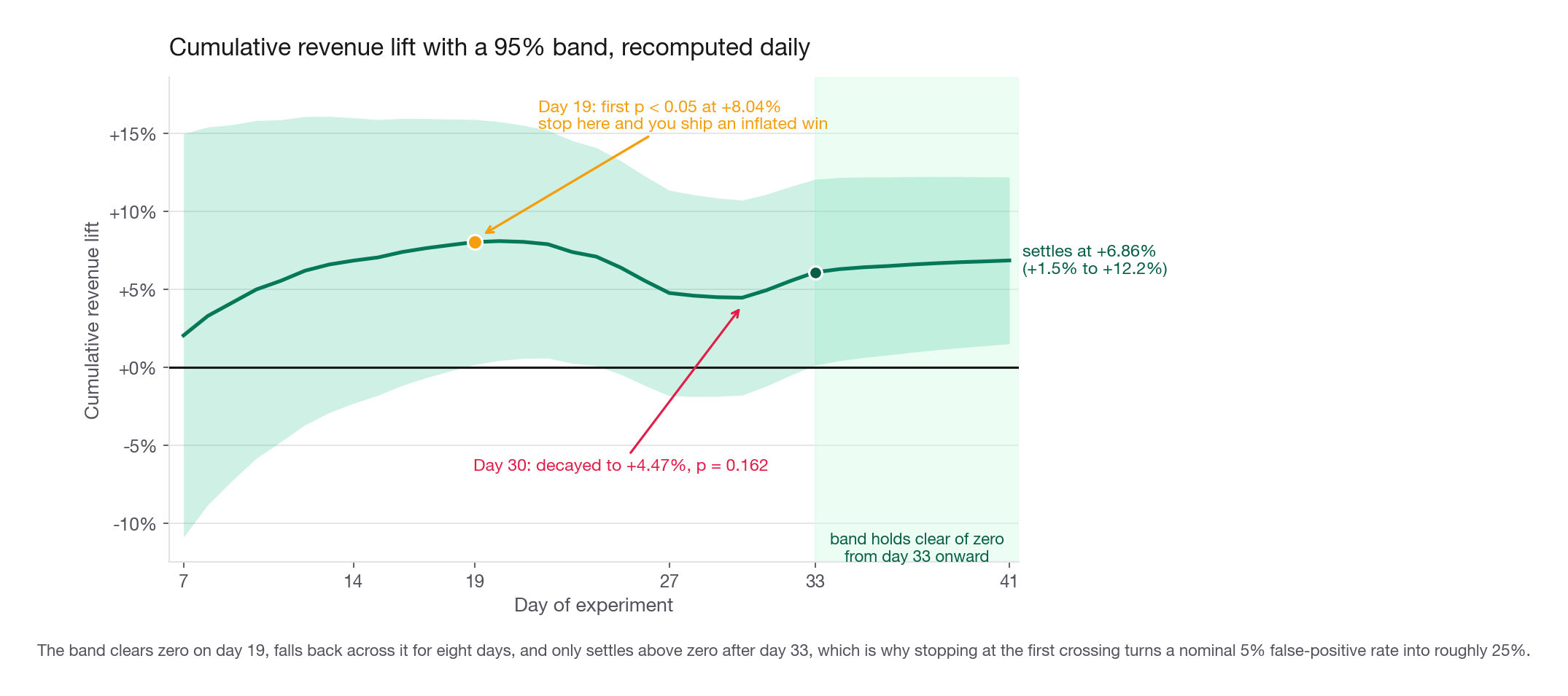
The cumulative estimate crosses p equal to 0.05 for the first time on calendar day 19, showing plus 8.04 percent. A team that had pre-committed to "stop when significant" ships 79 that afternoon and books an 8 percent revenue win.
Then look at what happens next. By day 27 the cumulative lift has decayed to plus 4.77 percent with p equal to 0.158. By day 30 it is plus 4.47 percent with p equal to 0.162. It does not recross 0.05 durably until day 33, and it settles at plus 6.86 percent. Across the 35 days examined, the cumulative p-value sits below 0.05 on 15 of them and above on 20. Peeking daily and stopping at the first crossing turns a nominal 5 percent false-positive rate into something closer to 25 percent, and in this run it would also have produced an effect estimate inflated by about a sixth.
Two acceptable answers to the stopping question:
Fixed horizon: compute the MDE before launch, pick the run length that reaches it, and look once. Here, if the business only cares about a lift of 10 percent or more, that is 22 days. If it cares about 5 percent, it is 89 days.
Sequential: if you truly need to monitor continuously, use a method built for it, an alpha-spending boundary or an always-valid confidence sequence. These are strictly wider than a fixed-horizon interval, which is the price of the option to stop early.
| Stopping rule | False positive rate | Effect estimate | Use when |
|---|---|---|---|
| Fixed horizon, one look | as designed | unbiased | you can pre-commit to a date |
| Peek daily, stop at p below 0.05 | roughly 25% here | inflated | never |
| Alpha spending with pre-set looks | as designed | mildly conservative | you need interim safety checks |
| Always-valid sequence | as designed | unbiased, wider band | dashboards anyone can read at any time |
Six weeks is also exactly six whole weeks, so weekday composition is identical across the run. B2B traffic is strongly weekly, and a 10-day or 17-day test overweights whichever days it happens to include. Always run in whole weeks.
The novelty argument cuts the other way here. Price has no novelty: nobody buys a seat because the number is unfamiliar. It does have a lag, since some teams who balk at 79 return a fortnight later, which biases short tests pessimistically.
Interview tip: When asked whether a test ran too long, answer with the minimum detectable effect at the achieved sample size. It converts an opinion into a number and it is the answer experimentation teams actually use.
The recommendation, and the growth tension
Here is where most candidates lose the thread. Revenue per visitor is up 6.9 percent and significant, so ship 79, right? Look at what else changed.
At 5,708 visitors a day, control produces 233.8 new accounts a day and treatment produces 172.8. That is 61 fewer teams onboarded every day, roughly 22,300 fewer per year. First-month revenue goes from about 40,357 a day to 43,124, a gain near 2,767 a day or a little over one million a year.
So the blanket price rise buys roughly one million in first-year billed revenue and costs 22,300 accounts. Whether that is a good trade depends on three things you cannot see in this dataset, and naming them is the point.
Expansion revenue. In seat-based B2B, accounts grow. A team that starts at 3 seats and adds 2 over a year is worth far more than its first invoice. Fewer accounts today compounds into a smaller expansion base for years.
Retention at the higher price. If teams that paid 79 churn faster, the first-month gain is a loan against future revenue. Nothing in a six-week acquisition test can tell you this.
Referral loops. Partner referral is Gridline's best-converting channel at 6.3 percent. Fewer accounts means fewer referrers, which shrinks the highest-quality channel with a lag.
Now compare against the segmented option the device interaction unlocked. Show 79 on mobile, keep 49 on desktop.
visitors_per_day = len(clean) / clean["day"].nunique()
mobile_share = (clean["device"] == "mobile").mean()
mob_t = clean[(clean["device"] == "mobile") & (clean["variant"] == "treatment")]
desk_c = clean[(clean["device"] == "desktop") & (clean["variant"] == "control")]
blend_arpv = (mobile_share * mob_t["revenue"].mean()
              + (1 - mobile_share) * desk_c["revenue"].mean())
blend_cr = (mobile_share * mob_t["converted"].mean()
            + (1 - mobile_share) * desk_c["converted"].mean())
print(round(visitors_per_day), round(blend_arpv, 3), round(100 * blend_cr, 3))
5708 7.671 3.902Revenue per visitor 7.67 against control's 7.07, a gain of 8.5 percent. Conversion 3.90 percent against 4.10 percent, so 222.7 accounts a day instead of 233.8, eleven fewer instead of 61. Before calling that a win on both axes, put intervals on both axes. The last two printed rows give the point estimate first, then its bounds.
bg = np.random.default_rng(SEED)
cells = {(dv, vr): clean.loc[(clean["device"] == dv) & (clean["variant"] == vr),
                             ["revenue", "converted"]].to_numpy()
         for dv in ["mobile", "desktop"] for vr in ["control", "treatment"]}
lifts = np.empty(4000)
for i in range(4000):
    r = {k: v[bg.integers(0, len(v), len(v))][:, 0].mean() for k, v in cells.items()}
    base = mobile_share * r[("mobile", "control")] + (1 - mobile_share) * r[("desktop", "control")]
    seg = mobile_share * r[("mobile", "treatment")] + (1 - mobile_share) * r[("desktop", "control")]
    lifts[i] = 100 * (seg / base - 1)
print(np.round(np.quantile(lifts, [0.025, 0.975]), 2))

dc, dt = cells[("desktop", "control")], cells[("desktop", "treatment")]
for j, scale in [(0, 100 / b.mean()), (1, visitors_per_day)]:
    gap = (1 - mobile_share) * (dc[:, j].mean() - dt[:, j].mean())
    s = (1 - mobile_share) * np.sqrt(dc[:, j].var(ddof=1) / len(dc) + dt[:, j].var(ddof=1) / len(dt))
    print(np.round(scale * (gap + np.array([0, -1.96, 1.96]) * s), 2))
[ 5.28 11.79]
[ 1.64 -2.58 5.86]
[49.94 42.9 56.98]The segmented lift over control is plus 8.5 percent, interval plus 5.3 to plus 11.8. Against the blanket 79 it is a different story: the revenue difference is plus 1.6 points, interval minus 2.6 to plus 5.9, so the two options are not separable on revenue at this sample size. That follows from where the difference lives. Segmented minus blanket is exactly the desktop share times the desktop treatment effect, reported above as minus 2.4 percent, interval minus 8.7 to plus 3.8, p equal to 0.447. A comparison built on a wash is a wash.
The account axis is where they separate: segmented delivers about 50 more accounts a day than the blanket rise, interval 43 to 57. So the honest sentence is that the segmented rollout is indistinguishable from the blanket rise on revenue and decisively better on volume, and volume carries the decision.
The recommendation to write: do not ship a blanket 79. Ship 79 to the mobile surface where the interaction is strong and the interval excludes zero, hold 49 on desktop where the effect is indistinguishable from nothing, and instrument 90-day retention and seat expansion on the mobile cohort before extending. If the organisation will not run segmented pricing, then holding at 49 is defensible: a 6.9 percent first-month gain with an interval that reaches down to 1.5 percent is not enough to justify a 26 percent cut in account acquisition without any retention evidence.
Then say what would change your mind, because interviewers ask. If 90-day retention at 79 is within two points of 49, the blanket rise becomes clearly correct. If accounts acquired at 79 expand seats at the same rate, the lifetime gap closes and the volume loss stops mattering. If mobile turns out to be a proxy for company size rather than buying context, price on size instead of device, which is both more durable and easier to defend to customers.
One practical warning to include: device-based price discrimination is visible, users compare notes, and the press coverage of it has been hostile. Package the same policy as a mobile-specific plan rather than one product at two prices.
Common traps
Leading with conversion rate. Reporting that conversion fell 26 percent as if it were the finding. It is mechanical. The fix: state up front that revenue per visitor is the decision metric and conversion is diagnostic.
Testing average order value. Comparing revenue per buyer across arms. Buyers are a post-treatment selection, so the comparison is not randomised. The fix: define every metric on the full assigned population, zeros included.
Skipping the price-versus-bucket cross-tab. Two columns encoding one fact is a planted bug. Here it hits 238 rows. The fix: cross-tabulate, report intent to treat on the full assigned population, and show the deletion as a sensitivity check.
Never plotting the daily series. The broken Friday moves the headline from p equal to 0.065 to 0.0115. The fix: plot conversion by day and arm first, and drop whole days rather than whole arms.
Winsorizing revenue at a fixed dollar cap. With unequal prices this censors the arms at different seat counts and manufactures a null. The fix: cap seats, or cap at within-arm percentiles.
Reading five channel p-values as five findings. One of five below 0.05 is what chance produces. The fix: fit the interaction, apply a multiplicity correction, and label unconfirmed segments as hypotheses.
Answering the duration question with intuition. "It felt long" is not analysis. The fix: report the minimum detectable effect at the achieved sample size and compare it to the observed effect.
Treating a first significance crossing as a stopping point. Here that fires on day 19 at an inflated plus 8.0 percent, then decays. The fix: fix the horizon in advance, or use a sequential method built for continuous monitoring.
Stopping at "ship 79". A recommendation with no account-volume number is not decision-ready. The fix: quantify both sides, revenue gained and accounts lost, and name the retention evidence you would need next.
Calling first-month revenue "revenue". In subscription businesses this is one invoice. The fix: label it explicitly and state that the lifetime comparison is unresolved.
Quick self-check
Answer each of these out loud, in under a minute, without looking at your notebook.
Why is average order value the wrong metric for comparing two price arms, and what is the name of the bias it introduces?
The observed revenue lift is plus 6.9 percent and the minimum detectable effect at the achieved sample size is 7.4 percent. What does that combination tell you about how much confidence to place in the point estimate?
Winsorizing revenue at a fixed dollar cap shrank the effect from 6.9 percent to 3.6 percent and erased its significance. Explain in one sentence why that check was invalid, using the seat arithmetic.
The cumulative p-value first drops below 0.05 on day 19 and rises back above it by day 27. What is the false positive rate of a daily-peeking stopping rule, and what are the two correct alternatives?
Partner referral shows plus 16.3 percent with p equal to 0.016. Should you price on it? Justify your answer with a number, not a preference.
Gridline gains about one million in first-year billed revenue and loses about 22,300 accounts per year under a blanket 79. Name the three quantities you would need in order to say whether that trade is positive, and say which of them this experiment can never measure.