2.1 Project: Diagnosing a Conversion Rate Problem
Find the core decision, design, or behavior signal.
Turn the lesson into a concise response blueprint.
Name the trap you would avoid in a real interview.
Use these checkpoints as your reading path before diving into the full lesson.
- 1What this lesson is for
- 2The brief
- 3Generate the working data
- 4Step 1: Sanity check before you get int...
- 5Step 2: The base rate decides which met...
Almost every candidate who gets this project builds a model that scores beautifully and then hands in a recommendation that cannot be acted on. The reason is a single column. This lesson walks the whole build for an online home-goods retailer, and the decision it prepares you for is the one that separates a pass from an offer: when your strongest predictor turns out to be something the product team cannot set, what do you do with it, and what do you tell them instead?
What this lesson is for
You get one flat table of web sessions, a binary purchase flag, and a prompt asking for recommendations to product and marketing. There is no join, no time series, no leakage from a second table. The whole challenge is interpretation, which is exactly why graders like it: nothing hides behind pipeline complexity.
Four things get scored here.
Did you notice the data problems before you modelled, and did you say what you would do about them beyond deleting rows?
Did you separate a real driver from a mix effect?
Did you recognise that the dominant feature is measured at the same time as the outcome, and therefore is not a lever?
Are the recommendations attached to a segment, a size, and a way to check whether they worked?
Item 3 is the whole project. The dataset is built so that one column carries almost all the predictive signal, and a candidate who reports "page views drive conversion, so get users to view more pages" has written a sentence that is simultaneously true, useless, and slightly embarrassing. A grader who works on this kind of product has read that sentence four hundred times.
Interview tip: When one feature holds more than about half the importance in a tree ensemble, stop modelling and ask when that feature is recorded relative to the label. Nine times out of ten the answer explains the score.
The brief
Lumen Home sells furniture, rugs, lighting, and kitchen goods online. Marketing wants to know where to move spend. Product wants to know what to fix on the site. You get an eight-week export of sessions, one row per session, with the outcome flagged at session level.
| Column | Type | Meaning | The trap in it |
|---|---|---|---|
market | category | Storefront the session hit, inferred from address | Confounded with channel mix and with device |
age | integer | Self-reported at account creation | Self-reported means unverified, and missing for guests |
first_session | 0 or 1 | 1 if the account was created during this visit | Reads like a user attribute, is really a traffic attribute |
acquisition_channel | category | Last touch before landing: paid social, organic search, direct, email | Last touch, not the channel that created the demand |
pages_viewed | integer | Pages loaded during the session | Counted across the whole session, including checkout |
purchased | 0 or 1 | Did an order complete in this session | Session grain, so a user who buys on visit three shows two failures |
Read the last column twice before writing any code. Three of those six traps are the project.
The questions attached to the brief are the usual pair: what explains the difference in conversion between groups of visitors, and what should the two teams do on Monday.
Generate the working data
Everything below runs on a deterministic build with that schema: 340,000 sessions across five storefronts over eight weeks. It bakes in a broken localised experience in one market, a channel mix that is badly unbalanced across markets, and, deliberately, a purchase flow that emits its own page views.
import numpy as np
import pandas as pd
SEED = 41
rng = np.random.default_rng(SEED)
N = 340000
MK = ["United States", "Mexico", "United Kingdom", "Canada", "Australia"]
market = rng.choice(MK, N, p=[.44, .21, .16, .12, .07])
mk = pd.Series({"United States": 0.0, "Mexico": -2.05, "United Kingdom": -0.06,
                "Canada": 0.04, "Australia": -0.12})[market].to_numpy()
soc = np.where(market == "Mexico", .62, .26)                  # Mexico is bought on paid social
u, rest = rng.random(N), 1 - np.where(market == "Mexico", .62, .26)
acquisition_channel = np.where(u < soc, "paid_social",
    np.where(u < soc + .46 * rest, "organic_search",
    np.where(u < soc + .76 * rest, "direct", "email")))
ch = pd.Series({"paid_social": -0.10, "organic_search": 0.0,
                "direct": 0.20, "email": 0.34})[acquisition_channel].to_numpy()
p_new = pd.Series({"paid_social": .86, "organic_search": .62,
                   "direct": .40, "email": .28})[acquisition_channel].to_numpy()
first_session = (rng.random(N) < p_new).astype(int)
age = np.clip(np.round(rng.gamma(11.0, 2.2, N) + 6).astype(int), 17, 79)
intent = (-0.30 + 0.70 * (1 - first_session) - 0.028 * (age - 28) + mk + ch
          + rng.normal(0, 0.85, N))
browse = 1 + rng.poisson(np.exp(1.35 + 0.42 * intent))        # pages seen before any cart
purchased = (rng.random(N) < 1 / (1 + np.exp(-(-6.5 + 0.62 * intent + 0.42 * browse)))).astype(int)
pages_viewed = browse + purchased * rng.integers(3, 6, N)     # checkout itself adds pages
sessions = pd.DataFrame({"market": market, "age": age, "first_session": first_session,
                         "acquisition_channel": acquisition_channel,
                         "pages_viewed": pages_viewed, "purchased": purchased})
sessions.loc[91744, "age"] = 137
sessions.loc[268301, "age"] = 104
Two lines in that generator are the lesson. browse is what a visitor looks at while deciding. pages_viewed, the column you are actually handed, is browse plus the pages the checkout flow itself renders. In a real log those extra pages are the cart, the shipping form, the payment step, and the confirmation screen. Nobody labelled them for you.
Step 1: Sanity check before you get interested
Open with shape, types, and the base rate, in that order. Three lines.
print(sessions.shape, sessions.dtypes.to_dict())
print("base rate", round(sessions.purchased.mean(), 5))
print(sessions.describe().round(2))
(340000, 6)
base rate 0.03482
age first_session pages_viewed purchased
mean 30.238 0.603 4.807 0.0348
std 7.278 0.489 3.082 0.1833
min 17.000 0.000 1.000 0.0000
50% 29.000 1.000 4.000 0.0000
max 137.000 1.000 37.000 1.0000A 3.5 percent session conversion rate for a considered-purchase retailer is completely ordinary, which is a useful thing to say out loud: it tells the grader you have a prior and that the export is not obviously corrupt. The median visitor is 29 and looks at four pages. Sixty percent of sessions belong to accounts created that same visit, which is high, and worth flagging as a possible paid-traffic artifact rather than a fact about the customer base.
Then the one value that does not belong.
odd = sessions[sessions.age > 90]
print(odd.to_string())
print("max plausible age:", sessions.loc[sessions.age < 90, "age"].max())
market age first_session acquisition_channel pages_viewed purchased
91744 Mexico 137 1 paid_social 1 0
268301 United States 104 1 paid_social 2 0
max plausible age: 77Two rows out of 340,000. Deleting them changes nothing measurable, and you should still spend a paragraph on them, because the paragraph is what is being graded, not the deletion.
The weak version reads: "There were two ages above 90 so I removed them." The stronger version reads: "Two sessions report ages of 137 and 104. Both are self-reported at account creation and both came in on paid social, which is where junk form fills concentrate. I dropped them because two rows cannot move a rate computed on 340,000. The reason to raise it anyway is that a field with no upper bound validation usually has a lower bound problem too, and if a share of visitors are typing whatever gets them past the form, then the age variable is noisier than its distribution suggests, and any age-based recommendation should be treated as directional."
That paragraph costs sixty seconds and shows three things: you know where bad data comes from, you sized the impact before acting, and you can tell a nuisance from a symptom.
Interview tip: Never write "I removed the outliers" without a sentence on what the outliers imply about the collection process. Cleaning is table stakes, inference about the pipeline is the point.
There is a second sanity check nobody runs: what is missing from the schema. There is no session timestamp, so you cannot check for a logging break mid-window or a weekday effect. There is no device, so any mobile hypothesis is unfalsifiable here. There is no order value, so every recommendation has to be sized in orders and converted to revenue with an assumed average. Write those three absences down in the notebook. When the recommendation later says "assume an average order of 96 USD," the grader already knows you did not have the column and chose an assumption on purpose.
Step 2: The base rate decides which metrics are allowed
At a 3.48 percent base rate, a model that predicts "nobody buys" for every session is 96.52 percent accurate. Any accuracy number you report has to be read against that floor, and most are not far above it. Fix the metric set before you fit anything.
The last line matters more than it looks. You will see below that one of the two models on this project predicts exactly zero positives at 0.5 while still being a genuinely useful ranker. A candidate who only reports the confusion matrix at the default threshold concludes the model is broken and throws away the better analysis.
Step 3: One driver at a time, before any model
The point of the univariate pass is not the plots. It is to reach the model with three hypotheses already written down, so the model confirms or refutes something rather than being asked to think for you.
Market: a twenty-fold gap is a bug, not a preference
clean = sessions[sessions.age < 90].copy()
by_market = (clean.groupby("market")
             .agg(sessions=("purchased", "size"), orders=("purchased", "sum"),
                  conv=("purchased", "mean"))
             .sort_values("conv"))
by_market["share_of_traffic"] = by_market.sessions / len(clean)
print(by_market.round(4).to_string())| Market | Sessions | Orders | Conversion | Share of traffic |
|---|---|---|---|---|
| Mexico | 71,523 | 159 | 0.22% | 21.0% |
| Australia | 23,555 | 882 | 3.74% | 6.9% |
| United Kingdom | 54,280 | 2,220 | 4.09% | 16.0% |
| United States | 149,962 | 6,591 | 4.40% | 44.1% |
| Canada | 40,680 | 1,966 | 4.83% | 12.0% |
Four markets sit inside a narrow band between 3.7 and 4.8 percent. The fifth is at 0.22 percent while taking a fifth of all traffic. That is not a difference in taste. Cultural preference does not produce a twenty-fold gap; a twenty-fold gap is what a broken funnel looks like.
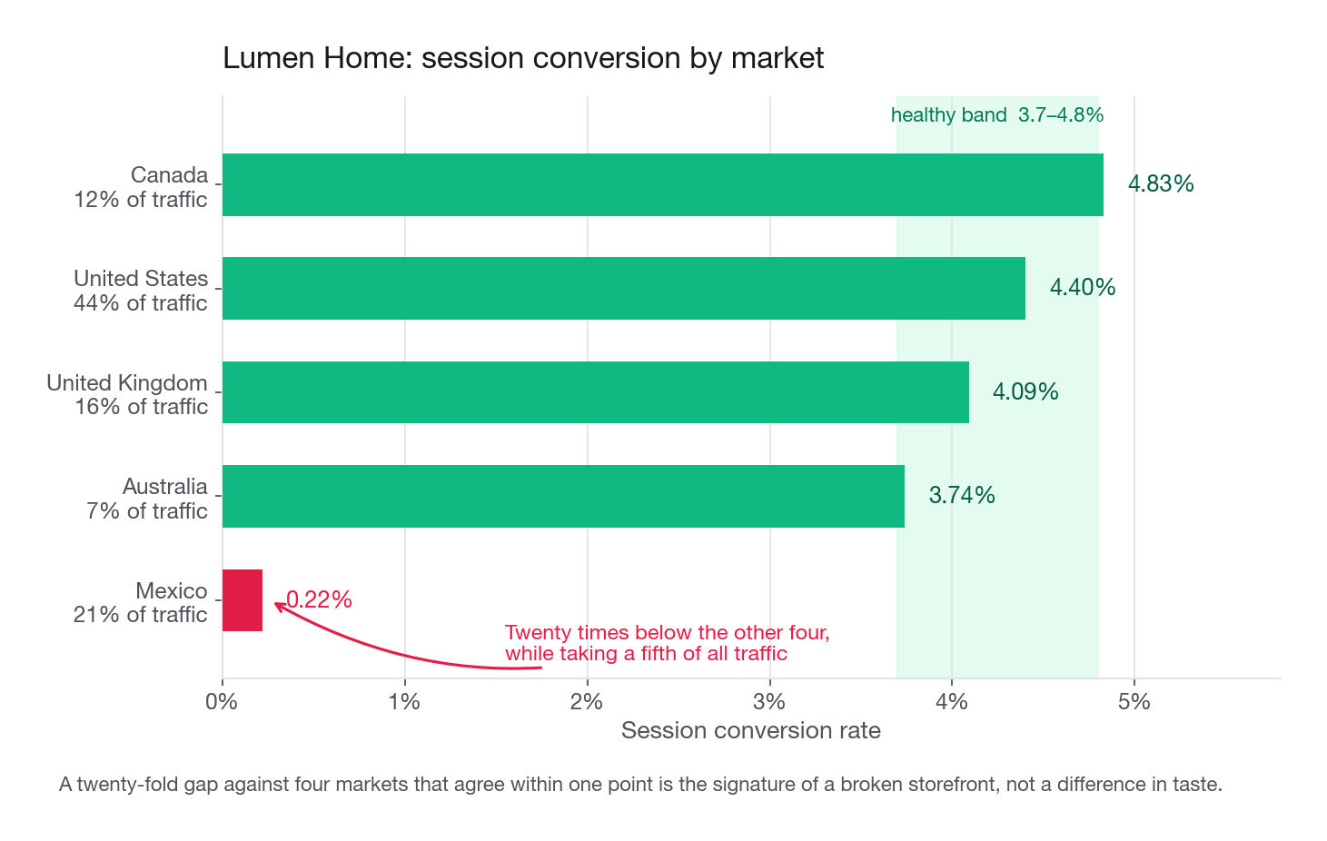
Before you claim a broken funnel, rule out the boring explanations. There are four and they take one query each.
Is it traffic quality? Check the share of sessions with a single page view and no purchase. If Mexico is mostly bounces, the problem is upstream of the site.
Is it a channel mix effect? Mexico may simply be bought through the worst channel.
Is it a new-versus-returning mix effect? A market with no returning base converts worse for reasons that have nothing to do with the storefront.
Is it browsing depth? If Mexico visitors look at the same number of pages and still do not buy, the drop is late in the funnel, near payment. If they look at fewer pages, the drop is early, near assortment or price.
mx = clean.market.eq("Mexico")
probe = clean.assign(is_mx=mx).groupby("is_mx").agg(
    conv=("purchased", "mean"),
    pct_new=("first_session", "mean"),
    pct_paid_social=("acquisition_channel", lambda s: (s == "paid_social").mean()),
    median_pages=("pages_viewed", "median"))
print(probe.round(4).to_string())
conv pct_new pct_paid_social median_pages
is_mx
False 0.0434 0.5739 0.2598 5.0
True 0.0022 0.7119 0.6182 2.0Mexico is 62 percent paid social against 26 percent elsewhere and skews new, so part of the gap is mix. What survives is still enormous: restrict to paid social on brand-new accounts and Mexico converts at 0.13 percent against 1.90 percent. Mix contributes, it does not explain.
The fourth column decides which half of the funnel you investigate, and it says the opposite of what most candidates assume. Median depth in Mexico is 2 pages against 5. Twenty-three percent of Mexico sessions are a single page with no order, against 4 percent elsewhere; only 2 percent reach seven or more pages, against 27 percent. That is not a bounce spike on a normal distribution, it is the whole distribution shifted left, which also means the first bullet does not fire cleanly: 23 percent bounces is high but it is not "mostly bounces", and traffic quality alone does not explain a market where the typical non-bouncing visitor stops at two pages.
By the decision rule three bullets up, that is the early funnel, not payment. Two checks confirm it. Conditional on depth, Mexico converts as well as or better than everywhere else at every level, 3.0 percent against 0.7 percent at seven pages and 33.8 percent against 10.9 percent at ten, whereas a checkout defect produces the reverse. And give Mexico the rest-of-world depth distribution at its own conditional rates and it converts at 6.4 percent, above the rest-of-world 4.3 percent. The gap lives entirely in how far people get.
So you still open the storefront in a browser, but you look at the landing page and the category listing, not the cart: an untranslated or half-broken landing page, prices rendered in the wrong currency on the listing, imagery or stock that never loads for that storefront, paid-social creative pointing somewhere that does not match its promise. Currency at checkout, local payment methods and shipping cost visibility move to a second pass, because nothing here implicates them yet.
Interview tip: When one segment is an order of magnitude worse, say the words "this looks like a defect, not a preference" and name the two or three defects you would look for. Interviewers are checking whether you would open the product, not just the notebook.
Acquisition channel: the mix effect that eats a naive answer
Here is the raw table, and here is why submitting it unadjusted costs you the project.
raw = clean.groupby("acquisition_channel").agg(
    sessions=("purchased", "size"), conv=("purchased", "mean"),
    pct_new=("first_session", "mean"))
raw["pct_mexico"] = clean.assign(m=mx).groupby("acquisition_channel")["m"].mean()
print(raw.round(4).to_string())| Channel | Sessions | Raw conversion | Share new accounts | Share from Mexico |
|---|---|---|---|---|
| paid_social | 113,958 | 1.50% | 86.0% | 38.8% |
| organic_search | 104,235 | 3.09% | 62.0% | 12.2% |
| direct | 67,686 | 5.05% | 40.1% | 12.0% |
| 54,121 | 6.39% | 28.1% | 12.0% |
Read naively: email converts four times better than paid social, so cut paid social and spend on email. That recommendation is wrong twice over. Paid social carries 39 percent of the broken market's traffic and 86 percent new accounts, while email is mostly people who already bought once and asked to hear from you. You are comparing a channel that manufactures strangers with one that harvests customers.
Standardise. Reweight every channel to the same market and new-versus-returning composition, which is a direct standardisation and takes eight lines.
strata = clean.groupby(["market", "first_session"]).size() / len(clean)
cell = clean.groupby(["acquisition_channel", "market", "first_session"])["purchased"].mean()
adj = {}
for chn in clean.acquisition_channel.unique():
    num = sum(w * cell[(chn, m, f)] for (m, f), w in strata.items() if (chn, m, f) in cell)
    den = sum(w for (m, f), w in strata.items() if (chn, m, f) in cell)
    adj[chn] = num / den
comp = pd.DataFrame({"raw": raw.conv, "standardised": pd.Series(adj)})
comp["raw_index"] = comp.raw / comp.raw["organic_search"]
comp["adj_index"] = comp.standardised / comp.standardised["organic_search"]
print(comp.round(4).to_string())| Channel | Raw conversion | Standardised | Raw index | Standardised index |
|---|---|---|---|---|
| paid_social | 1.50% | 2.62% | 0.49 | 0.90 |
| organic_search | 3.09% | 2.93% | 1.00 | 1.00 |
| direct | 5.05% | 3.88% | 1.63 | 1.33 |
| 6.39% | 4.53% | 2.07 | 1.55 |
The email advantage over paid social falls from 4.3x to 1.7x. Most of what looked like channel quality was composition. There is still a real ordering left, and now you can defend it. That single table is worth more than any model on this project, and it takes ten minutes.
Interview tip: Say the phrase "how much of this gap survives standardisation" out loud during the interview. It is the fastest signal that you have run comparisons before, and it turns a marketing question into a measurement question.
New versus returning, and the age slope
Returning visitors convert at 6.11 percent against 1.74 percent for accounts created in the session, a 3.5x gap on 135,009 versus 204,989 sessions. That is real and stable across markets. It also tells marketing very little on its own, because you cannot decide to have more returning users this quarter; you can only decide to bring back the ones you already have.
Age slopes down cleanly.
| Age band | Sessions | Share of traffic | Conversion |
|---|---|---|---|
| 17 to 24 | 77,025 | 22.7% | 4.73% |
| 25 to 29 | 93,105 | 27.4% | 3.80% |
| 30 to 34 | 82,643 | 24.3% | 3.19% |
| 35 to 39 | 50,151 | 14.8% | 2.49% |
| 40 to 49 | 32,873 | 9.7% | 2.12% |
| 50 and over | 4,201 | 1.2% | 1.40% |
The monotone decline is the kind of finding candidates over-claim. Two honest caveats belong next to it. Age is self-reported and unverified, so the youngest band is partly people who typed a number. And age correlates with device, with time of day, and with which campaigns reached them, none of which are in this table. The defensible version of the claim is that the site converts younger visitors better and you cannot tell from this data whether that is about the assortment, the price points, or the checkout experience on the devices those groups use.
Step 4: The variable that eats the project
Now the column the whole thing hinges on.
depth = clean.groupby("pages_viewed")["purchased"].agg(["size", "mean"]).head(14)
print(depth.round(5).to_string())
print("buyer mean pages", round(clean.loc[clean.purchased == 1, "pages_viewed"].mean(), 2))
print("non-buyer mean pages", round(clean.loc[clean.purchased == 0, "pages_viewed"].mean(), 2))
pages_viewed size conv
1 26994 0.00000
2 49561 0.00000
3 56614 0.00000
4 53329 0.00017
5 44312 0.00099
6 34038 0.00267
7 24267 0.00762
8 16409 0.02365
9 10867 0.05365
10 6968 0.11079
11 4489 0.21608
12 2870 0.39303
buyer mean pages 14.11
non-buyer mean pages 4.47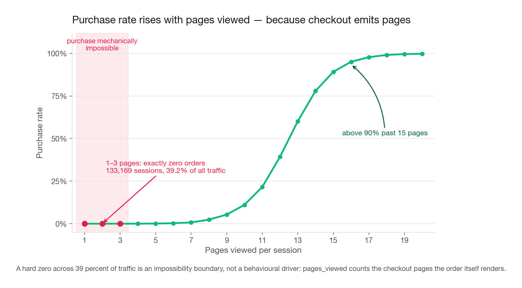
An S-curve this steep looks like the most actionable finding on the page. It is the opposite. Look at the top three rows: 133,169 sessions, 39.2 percent of all traffic, and exactly zero orders. Not a low rate. Zero. A genuine behavioural driver does not produce a hard impossibility boundary.
The boundary is mechanical. A completed order renders the cart, the address step, the payment step, and the confirmation. Those pages land in pages_viewed because the column counts every page in the session, and nobody split browse pages from checkout pages when the export was written. So a session with three pages cannot contain a purchase in the same way that a receipt cannot be printed before the sale.
This is not leakage in the textbook sense, where a column is derived from the label. It is worse in practice, because it is subtle enough to survive review: pages_viewed is a legitimate metric, it is measured in the same session, and it is partly caused by the outcome it is being used to predict.
The test that tells a lever from a proxy
Run every candidate feature through two questions before you let it into a recommendation.
pages_viewed fails timing, fails control, and fails the counterfactual spectacularly. You can raise average pages per session tomorrow by paginating the category listing into three pages instead of one, and conversion will fall. A metric you can move in the wrong direction while moving the target the other way is a diagnostic, not a lever.
Compare the other columns against the same test.
| Feature | Determined before outcome | Team can set it | Verdict |
|---|---|---|---|
market | Yes | Yes, product owns the storefront | Lever |
acquisition_channel | Yes | Yes, marketing owns the spend split | Lever |
first_session | Yes | Partly, through retention and lifecycle | Weak lever |
age | Yes | No, only targeting can shift the mix | Targeting variable |
pages_viewed | No | No | Proxy, and partly an outcome |
Three good repairs exist, in order of preference. First, ask the engineer for a flag separating pre-cart pages from checkout pages, and refit on pre-cart depth only, which is a real engagement measure. Second, if you cannot get that, keep pages_viewed out of the driver model and use it only as a segmentation field for sessions that did not convert. Third, if you must keep it, censor it: cap depth at the last page before any cart event. In a take-home you do not have the engineer, so you say what you would ask for, and you build the second option.
Interview tip: The sentence that lands here is "this feature is contemporaneous with the outcome, so it belongs in a diagnostic, not in a recommendation." Say it before the interviewer has to ask what is wrong with your top feature.
Step 5: Fit a model, and say why in two sentences
Model choice on this project is nearly free, because the deliverable is insight rather than a production score. Justify it briefly and move on.
For this build, take a forest for the shape and a logistic regression alongside it for signed effects. The forest gives you importance ordering and partial dependence; the regression gives you an odds ratio you can quote in a sentence. Both belong on the lever set, so the regression waits for Step 6 to drop the contemporaneous column.
from sklearn.model_selection import train_test_split
from sklearn.ensemble import RandomForestClassifier
from sklearn.metrics import roc_auc_score, average_precision_score, confusion_matrix

X = pd.get_dummies(clean.drop(columns="purchased"),
                   columns=["market", "acquisition_channel"])
y = clean.purchased
Xtr, Xte, ytr, yte = train_test_split(X, y, test_size=0.30, random_state=7, stratify=y)

def fit_report(cols, tag):
    rf = RandomForestClassifier(n_estimators=160, min_samples_leaf=40,
                                n_jobs=-1, random_state=7)
    rf.fit(Xtr[cols], ytr)
    p = rf.predict_proba(Xte[cols])[:, 1]
    tn, fp, fn, tp = confusion_matrix(yte, (p >= 0.5).astype(int)).ravel()
    print(tag, "AUC %.4f" % roc_auc_score(yte, p),
          "PR-AUC %.4f" % average_precision_score(yte, p),
          "acc %.4f" % ((tn + tp) / len(yte)), "tp", tp, "fn", fn, "fp", fp)
    return rf, p
Fit the naive version first, the one that keeps every column.
rf_all, p_all = fit_report(list(X.columns), "with pages_viewed:")
imp = pd.Series(rf_all.feature_importances_, index=X.columns).sort_values(ascending=False)
print(imp.head(5).round(4).to_string())
with pages_viewed: AUC 0.9797 PR-AUC 0.7968 acc 0.9826 tp 2341 fn 1204 fp 569
pages_viewed 0.9656
first_session 0.0105
age 0.0100
market_Mexico 0.0057
acquisition_channel_email 0.0024An AUC of 0.98 on a 3.5 percent target. Precision 0.80 and recall 0.66 at the default cut. Accuracy 98.26 percent against a 96.52 percent floor, so the accuracy gain is 1.74 points, which is the first hint that the headline number is less impressive than it reads.
And one feature holds 96.6 percent of the importance. That is the alarm. On a real driver set you expect the top feature somewhere between 20 and 45 percent. When a single column crosses 90 percent, either the problem is genuinely one-dimensional or the column is downstream of the label. Here you already know which.
Step 6: Refit without the proxy, and read what is left
Drop the column and fit again. The score falls a long way, and everything that remains is something a team can act on.
cols = [c for c in X.columns if c != "pages_viewed"]
rf_lev, p_lev = fit_report(cols, "levers only:")
print(pd.Series(rf_lev.feature_importances_, index=cols)
      .sort_values(ascending=False).head(6).round(4).to_string())
levers only: AUC 0.7286 PR-AUC 0.0776 acc 0.9652 tp 0 fn 3545 fp 0
first_session 0.3080
age 0.3074
market_Mexico 0.1784
acquisition_channel_paid_social 0.0570
acquisition_channel_email 0.0506
acquisition_channel_organic_search 0.0248Two things to explain, and both are worth points.
First, the model predicts zero positives at a 0.5 threshold. Its accuracy is exactly the all-negative baseline. A candidate who stops here writes "the model failed." It did not fail. At a 3.5 percent base rate almost no session reaches a 50 percent predicted probability, because almost no session is more likely than not to convert. The threshold is wrong, not the model. Score the ranking instead.
Second, an AUC of 0.729 is the honest ceiling of what these five columns can say about a single session. Say so plainly. A grader trusts 0.73 with a clear explanation far more than 0.98 with a proxy inside it.
dec = pd.DataFrame({"p": p_lev, "y": yte.values})
dec["decile"] = pd.qcut(dec.p, 10, labels=False, duplicates="drop")
out = dec.groupby("decile").agg(sessions=("y", "size"), conv=("y", "mean"))
out["lift"] = out.conv / yte.mean()
print(out.round(4).to_string())| Decile | Sessions | Conversion | Lift versus base |
|---|---|---|---|
| 10 (top) | 10,144 | 9.50% | 2.73x |
| 9 | 10,180 | 6.84% | 1.97x |
| 8 | 10,274 | 5.09% | 1.46x |
| 7 | 10,200 | 3.93% | 1.13x |
| 4 to 6 | 30,537 | around 2.4% | 0.70x |
| 3 | 10,221 | 1.45% | 0.42x |
| 2 | 10,234 | 0.31% | 0.09x |
| 1 (bottom) | 10,210 | 0.32% | 0.09x |
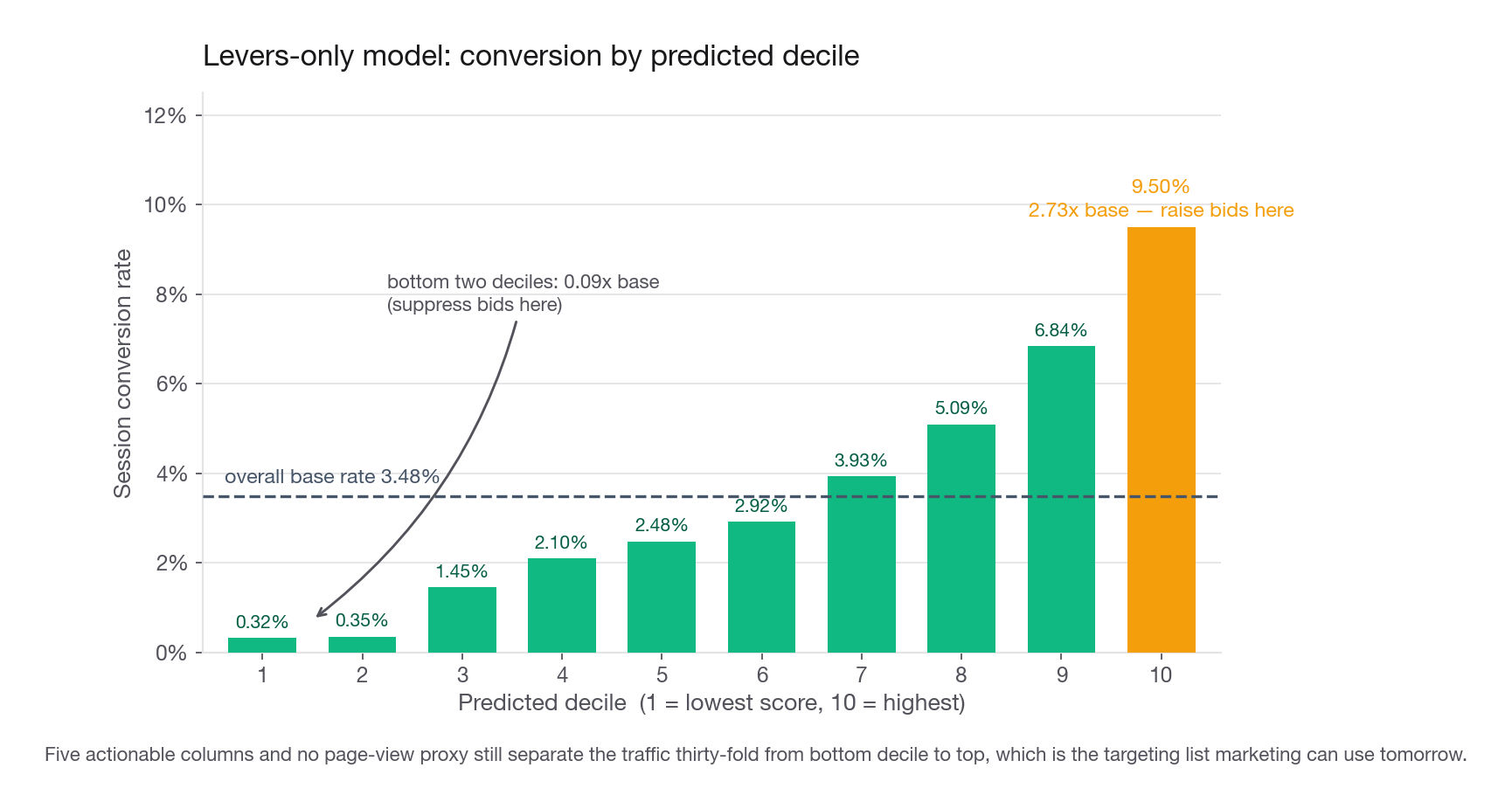
That table is the deliverable. Without a single page-view column, five ordinary attributes separate the traffic by a factor of thirty between the bottom and top decile. Before you hand it to marketing, ask what is actually in the two ends, because a decile score is only as honest as its composition.
The bottom is not a blend of five attributes. It is 87.5 percent Mexico, and it holds 84 percent of every Mexico session in the test set: a Mexico detector wearing a model's clothes. The top is genuinely multi-attribute, 98 percent returning accounts, average age 27, 80 percent email or direct, no Mexico at all. Only one of those ends is a clean bidding instruction.
The obvious instruction, "suppress bids on the bottom two deciles and raise them on the top two", is not the one to write. Suppressing the bottom means "stop buying Mexico traffic", which collides with the largest recommendation on your board. The Mexico sizing in Step 7 is computed on current Mexico session volume, Mexico is 62 percent paid social, and the verification plan needs half of that traffic still flowing to read the fix at two weeks. Cut the spend first and you shrink the opportunity you just sized and starve the test that would have confirmed it. So the score ships with a carve-out and an order of operations: hold Mexico out of bid suppression until the storefront fix has landed and been measured, then revisit.
The other end needs its own arithmetic. Inside paid social only 1.65 percent of sessions reach the top two deciles, 562 of 34,082, because the good deciles are mostly email and direct traffic no auction is bidding for. "Raise bids on the top two" is close to a no-op inside the channel the recommendation names; the move that survives is reallocating budget across channels, not re-bidding within paid social. And say how it deploys: geo, channel, an age bracket and prospecting versus retargeting are ad-platform targeting dimensions, not an impression-level score, so this is segment-level bid adjustment and should be described that way rather than promised as real-time scoring.
Reading partial dependence without over-claiming
Partial dependence answers one narrow question: holding everything else at its observed distribution, how does the predicted rate move as this one feature moves? It is a picture of the model, not of the world. Compute it rather than eyeballing a plot, and for a one-hot category set the whole block at once: toggling a single dummy leaves the row all-zero or double-hot, a state the model never saw, and here that returns a spread 40 percent too small.
def cat_pdp(model, base, prefix):
    block = [c for c in base.columns if c.startswith(prefix)]
    out = {}
    for c in block:
        tmp = base.copy()
        for cc in block:
            tmp[cc] = (cc == c)
        out[c[len(prefix):]] = model.predict_proba(tmp)[:, 1].mean()
    return pd.Series(out).sort_values()

print((cat_pdp(rf_lev, Xte[cols], "acquisition_channel_") * 100).round(2).to_string())
print()
print((cat_pdp(rf_lev, Xte[cols], "market_") * 100).round(2).to_string())
paid_social 2.65
organic_search 2.91
direct 3.92
email 4.62
Mexico 0.28
Australia 3.58
United Kingdom 4.06
United States 4.17
Canada 4.59Three readings from this fit are worth quoting.
Market: Mexico sits between 3.3 and 4.3 points below the other four, 3.8 points below their average, and the four span only 1.0 point between them. That is consistent with one broken storefront rather than a spectrum of market quality.
Age: a smooth decline of roughly 3 points from the youngest to the oldest band, with no kink. No kink matters, because a kink would suggest a device or an interface threshold rather than a preference gradient. Read it by band and not year by year, though: only 1.2 percent of sessions are 50 or older, so the single-year curve wobbles above the 40s even while the band-level decline stays monotone.
Channel: the surviving spread after conditioning is 1.97 points between email and paid social, against 1.90 points from the direct standardisation you ran in Step 3. Two independent methods landing 0.06 points apart is worth a sentence in the write-up, and it is a much stronger sentence than either number on its own.
Interview tip: State that partial dependence describes the model, then give the number anyway. Candidates who only give the caveat sound hedging, and candidates who only give the number sound naive.
The signed version: one sentence per driver
Partial dependence gives you shape on the probability scale, not a signed effect you can say out loud in a meeting. That is the second model promised in Step 5, and it costs six lines on the same lever set.
One setup detail decides whether the output is readable. The get_dummies call above keeps every level of market and acquisition_channel, which is fine for a forest and rank-deficient for a regression: fit on that matrix and market_United States comes back at an odds ratio of 1.32, which reads as "the American storefront lifts odds by a third" and is pure artifact of an absent baseline. Build a separate matrix with an explicit reference level per block, and leave the forest's X alone so the earlier output still reproduces.
from sklearn.linear_model import LogisticRegression

Xlr = pd.get_dummies(clean.drop(columns=["purchased", "pages_viewed"]),
                     columns=["market", "acquisition_channel"])
Xlr = Xlr.drop(columns=["market_United States",
                        "acquisition_channel_organic_search"]).astype(float)
Ltr, Lte, ytr2, yte2 = train_test_split(Xlr, y, test_size=0.30,
                                        random_state=7, stratify=y)
lr = LogisticRegression(max_iter=2000, C=1e6).fit(Ltr, ytr2)
print(pd.Series(np.exp(lr.coef_[0]), index=Xlr.columns).round(3).to_string())
print("LR AUC %.4f" % roc_auc_score(yte2, lr.predict_proba(Lte)[:, 1]))
age 0.961
first_session 0.361
market_Australia 0.846
market_Canada 1.116
market_Mexico 0.068
market_United Kingdom 0.969
acquisition_channel_direct 1.393
acquisition_channel_email 1.620
acquisition_channel_paid_social 0.915
LR AUC 0.7467Three sentences come out of that, and each names its baseline, because an odds ratio without a reference category is unreadable.
Holding age, returning status and channel fixed, a Mexico session has 0.068 times the odds of an otherwise identical United States session, roughly one fifteenth.
A returning account has 2.77 times the odds of a first-session account, which is 0.361 inverted so the comparison runs in the direction anyone cares about.
Age carries 0.961 per year, which compounds to 0.675 over a decade, so ten more years of self-reported age costs about a third of the odds.
Then the sentence that justifies fitting two models: the regression's test AUC is 0.7467, slightly above the forest's 0.7286. When an additive log-odds model matches a forest on ranking, the relationships really are close to additive, which is the condition the tradeoff matrix names for preferring logistic regression. The two agree, so the model choice was defensible rather than a coin flip.
One caveat belongs next to those numbers. At a 3.5 percent base rate an odds ratio and a risk ratio nearly coincide, so "fifteen times worse odds" and "fifteen times worse conversion" are interchangeable here. That is a property of the low base rate. Quote an odds ratio as a rate change on a 30 percent outcome and you will be badly wrong, so say which scale you are on.
Interview tip: Name the reference category in the same breath as any odds ratio, and say whether the base rate is low enough for it to double as a rate ratio. That clause is the difference between a stakeholder using your number and misusing it.
Step 7: Turn drivers into recommendations with a size attached
A recommendation without a number is an opinion. Size each one before you write it.
The Mexico fix is the largest single item on the board.
WEEKS, AOV = 8, 96.0
annualise = 52 / WEEKS
mx_rows = clean[clean.market == "Mexico"]
row_rest = clean[clean.market != "Mexico"]
target = row_rest.purchased.mean() / 2          # half of rest-of-world, deliberately modest
gain = (target - mx_rows.purchased.mean()) * len(mx_rows) * annualise
print("Mexico sessions per year %.0f" % (len(mx_rows) * annualise))
print("orders today %.0f" % (mx_rows.purchased.sum() * annualise))
print("incremental orders %.0f, revenue %.0f USD" % (gain, gain * AOV))
Mexico sessions per year 464893
orders today 1034
incremental orders 9061, revenue 869843 USDRoughly 870,000 USD a year, and that is on a deliberately conservative target of half the rest-of-world rate, not parity. The assumption is stated and deliberately pessimistic: at full parity the number roughly doubles. Quote the low figure and mention the range.
The second item comes from the proxy you set aside. Sessions that browsed deeply and did not buy are not a modelling artifact, they are a list.
pool = clean[(clean.purchased == 0) & (clean.pages_viewed >= 7)]
print(len(pool), "deep non-converting sessions, %.1f%% of traffic"
      % (100 * len(pool) / len(clean)))
print(pool.market.value_counts(normalize=True).round(3).to_string())
63476 deep non-converting sessions, 18.7% of traffic
United States 0.556 United Kingdom 0.191 Canada 0.156 Australia 0.077 Mexico 0.020Nearly one session in five involved seven or more pages and no order. Those visitors demonstrated intent and left. That is the highest-quality remarketing audience on the site, and it exists whether or not pages_viewed is a causal lever, because using it to segment does not require it to cause anything.
Read the market column too: Mexico is 2.0 percent of this pool while being 21 percent of traffic. Almost nobody there gets deep enough to qualify, which is Step 3's early-funnel finding arriving from the far end, and why this audience is not worth building in Mexico until the storefront fix lands.
Here is the board, with an owner and a check on every line.
| Recommendation | Owner | Sizing | Confidence | How you would verify |
|---|---|---|---|---|
| Audit the top of the Mexico funnel: landing page and category listing render, translation, listing-price currency, paid-social landing quality | Product | About 9,100 orders per year, near 870,000 USD | High, a 20x gap is not preference | Ship the fix to half of Mexico traffic and read conversion at two weeks |
| Rebalance spend across channels using the decile score, holding Mexico out until the storefront fix is measured | Marketing | 20,444 test-set sessions at 0.09x lift, about 68,000 sessions over the eight-week window | Medium, ranking is proven, spend response is not | Holdout geography, compare cost per order over four weeks |
| Build a remarketing audience from deep non-converting sessions | Marketing | 63,476 sessions in eight weeks, 18.7% of traffic | Medium to high, intent is demonstrated | Randomly withhold 30 percent of the audience, compare return rate |
| Investigate why conversion declines with age before targeting on it | Product | 26 percent of traffic is over 34 at 2.3% conversion | Low, confounded with device and assortment | Add a device column to the export, then re-run the age slope within device |
| Stop reporting pages per session as a conversion driver | Both | No revenue, prevents a bad roadmap item | High | Show the zero-order region below four pages once, and it settles |
The last row is not filler. Half the value of this project is preventing a quarter of work aimed at raising a metric that partly measures the outcome it is supposed to cause.
What the write-up actually contains
Three pages. Page one: the question, the base rate, the two data problems and what you did, and the single sentence that Mexico is a defect. Page two: the market table, the standardised channel table, and the pages-viewed curve with the zero region marked. Page three: the recommendation board above, and a short paragraph on what you would ask engineering for.
Nowhere in those three pages is there a hyperparameter. The model earns two sentences: what it was, and that dropping the contemporaneous feature moved AUC from 0.98 to 0.73, which is the honest number.
Common traps
Reporting 98 percent accuracy as a headline. At a 3.48 percent base rate the do-nothing model scores 96.52 percent. Always print the baseline on the same line as the score, and prefer PR AUC or decile lift for the headline.
Believing the raw channel table. Paid social looks 4.3x worse than email until you standardise for market and returning-user mix, after which it is 1.7x worse. The fix is eight lines of direct standardisation, and it changes the recommendation.
Treating the strongest predictor as the strongest lever. Importance ranks how useful a column is for prediction. It says nothing about whether anyone can set it. Run the timing and control questions on your top feature before it reaches a slide.
Concluding the levers-only model failed because it predicted no positives at 0.5. The default threshold is an artifact of a library, not a property of your problem. Evaluate the ranking, then choose a cut from what the decision costs.
Deleting the impossible ages and saying nothing. The deletion is correct and worth zero points. The observation that an unvalidated self-reported field is probably noisy throughout, and that age-based recommendations should be treated as directional, is worth several.
Recommending "increase engagement" as an action. It names no change, no owner, and no measurement. Replace it with a specific storefront fix, a specific audience, or a specific bid change, each with a number attached.
Sizing with an unstated average order value. The export has no revenue column. Pick a figure, write "assume 96 USD average order," and show the number both ways if the decision is close to a boundary.
Claiming causality from partial dependence. The curves describe the fitted model under an observed covariate distribution. Quote the magnitude, name the confound you could not rule out, and say which experiment would settle it.
Building the model before the univariate pass. The market table alone contains the largest finding in the project. If a model is the first thing you fit, you will spend your remaining hours tuning a score instead of explaining a twenty-fold gap.
Forgetting the grain. One row is one session, not one user. A visitor who browses twice and buys on the third visit contributes two zeros and one one. Every rate you quote is per session, and the write-up should say so once, because the same numbers mean something different per user.
Quick self-check
Answer these aloud, in full sentences, the way you would to an interviewer.
The base rate is 3.48 percent and your model is 98.3 percent accurate. In two sentences, why is that not a good headline, and what do you report instead?
Sessions with three or fewer pages viewed have exactly zero orders, and they are 39 percent of traffic. What does an exact zero tell you that a very low rate would not?
Raw conversion is 6.39 percent on email and 1.50 percent on paid social. After standardising to a common market and returning-user mix it is 4.53 against 2.62. Which number goes in the recommendation, and what do you say about the other?
Your top feature holds 96.6 percent of the forest's importance. Walk through the two questions you ask about that feature, and what you do with it after both answers come back negative.
The levers-only model predicts zero positives at a 0.5 threshold. Explain to a marketing manager, without the word "threshold," why the model is still useful.
Mexico is 21 percent of traffic at 0.22 percent conversion. Size the opportunity, state the assumption you made about average order value, and name the first thing you would check to confirm the cause before anyone builds anything.