3.2 Challenge: Parsing Search URLs Into a Clean Dataset
Find the core decision, design, or behavior signal.
Turn the lesson into a concise response blueprint.
Name the trap you would avoid in a real interview.
Use these checkpoints as your reading path before diving into the full lesson.
- 1What this lesson is for
- 2The brief
- 3The fields hiding in the URL
- 4Build the working copy
- 5Step 1: parse the query string without...
Roamly is a vacation-rental search product that has been shipping for two years and instrumenting for none of them. There is no events table, no search log, no warehouse. What exists is a text file scraped off the load balancer: one line per search, each a raw URL with every filter encoded in the query string. Your task is to turn that file into something queryable, then use it to answer a question the product team actually cares about, which city has the worst search ranking. The parsing is the visible half of the work and the cheap half. The expensive half is deciding what "worst search ranking" means as a number, and then noticing that the first number you compute ranks the cities wrong.
What this lesson is for
Two skills get tested here, and candidates over-invest in the first.
The first is mechanical: pull structured fields out of semi-structured text without silently dropping data. Early-stage companies really do store behavioral data this way, and scraping and log reconstruction reduce to the same problem. It is worth maybe a quarter of the score.
The second is judgment: given a column called result_page, invent a metric a ranking team can be held accountable to, defend it against the obvious alternatives, then check whether the ranking survives the fact that different cities get asked different questions. That is where the interview is won.
Candidates hand in a clean parser, a clean table, one line of groupby, and a conclusion that names the wrong city. The parser is not what failed them. A per-city rate computed over a mix that differs by city is a mix comparison, not a quality comparison, and search depth is one of the most mix-sensitive quantities in any marketplace. By the end of this page you will have a parse that survives review, a metric with a stated decision behind it, an interval around every number, and a corrected ranking that flips the naive answer.
Interview tip: When a prompt says "create a metric", it is asking you to defend a choice, not to produce a formula. Say the decision the metric drives in your first sentence, then the formula.
The brief
Roamly wants three things.
A clean table where each row is one search, each column is one query parameter, and cells hold the value the user selected.
The searches that used more than one property filter, and how common that is.
A metric based on how far into the result pages users go, plus the city that scores worst on it.
The fields hiding in the URL
Every Roamly search URL starts with the same prefix and then carries some subset of these parameters. Three are always present because the search form will not submit without them. The rest appear only when the user touched that control, which is the single most important structural fact about this data.
| Parameter | Meaning | Always present |
|---|---|---|
stay.checkin | Arrival date, ISO format | Yes |
stay.checkout | Departure date, ISO format | Yes |
stay.city | Destination, percent-encoded free text | Yes |
stay.guests | Adults sharing the booking | Yes |
stay.result_page | Deepest result page the user reached | Yes |
stay.kids | Children in the party, absent when zero | No |
stay.priceFloor | Minimum nightly rate in USD | No |
stay.priceCeiling | Maximum nightly rate in USD | No |
stay.instantBook | Checkbox, value yes when ticked | No |
stay.rating_min | Minimum guest rating, 1 to 5 scale | No |
stay.promoCode | Checkbox, yes when a code was applied | No |
stay.features | Property filter checkbox, repeats once per box ticked | No |
Read the last row twice. stay.features is the only parameter that can repeat within one URL, because the filter panel is a set of checkboxes and each ticked box serializes as its own key. A user who wants a pool and a washer generates stay.features=pool&stay.features=washer. Any parser that builds a key-to-value dictionary keeps one and discards the other without warning. That silent loss is the classic failure here, and it corrupts question two directly.
The possible feature values are wifi, parking, pool, kitchen, pets_ok, and washer.
Build the working copy
The block below manufactures the raw file. It is deterministic, so every count and rate quoted on this page reproduces exactly. Under the hood it gives each city its own baseline tendency to send users past page one, and it also gives each city its own query mix, which is the trap we will spring in step five. Run it once and keep raw in memory.
import numpy as np
import pandas as pd

SEED = 4471902
rng = np.random.default_rng(SEED)
N = 48000
BASE = "https://roamly.example/search/stays?"
FEATS = ["wifi", "parking", "pool", "kitchen", "pets_ok", "washer"]
CFG = {   # city -> volume share, deep-search intercept, filter mix, guest range
    "Kyoto%2C+Japan":                   (.18, -2.30, [.62, .28, .08, .02], (1, 5)),
    "Lisbon%2C+Portugal":               (.31, -1.85, [.60, .29, .09, .02], (1, 6)),
    "Austin%2C+Texas%2C+United+States": (.27, -1.40, [.55, .30, .12, .03], (1, 6)),
    "Medellin%2C+Colombia":             (.15, -0.60, [.63, .27, .08, .02], (1, 5)),
    "Reykjavik%2C+Iceland":             (.09, -1.05, [.18, .30, .32, .20], (4, 9)),
}
OPT = [("stay.priceCeiling", .22, lambda: rng.integers(70, 420)),
       ("stay.priceFloor", .11, lambda: rng.integers(30, 120)),
       ("stay.instantBook", .19, lambda: "yes"),
       ("stay.rating_min", .16, lambda: round(float(rng.uniform(3.0, 4.8)), 1)),
       ("stay.promoCode", .04, lambda: "yes")]

city = rng.choice(list(CFG), N, p=[CFG[c][0] for c in CFG])
ci = np.datetime64("2026-03-01") + rng.integers(0, 150, N).astype("timedelta64[D]")
co = ci + rng.integers(1, 10, N).astype("timedelta64[D]")
guests = rng.integers(*np.array([CFG[c][3] for c in city]).T)
kids = np.where(rng.random(N) < 0.27, rng.integers(1, 4, N), 0)
nfeat = np.array([rng.choice(4, p=CFG[c][2]) for c in city])
z = (np.array([CFG[c][1] for c in city]) + .55 * nfeat
     + .35 * (guests + kids >= 6) + .20 * ((co - ci).astype(int) >= 7))
page = rng.geometric(1 - 1 / (1 + np.exp(-z)))

urls = []
for i in range(N):
    opt = [f"stay.kids={kids[i]}"] if kids[i] else []
    opt += [f"{k}={fn()}" for k, p, fn in OPT if rng.random() < p]
    opt += [f"stay.features={f}" for f in rng.choice(FEATS, nfeat[i], replace=False)]
    rng.shuffle(opt)
    q = [f"stay.checkin={ci[i]}", f"stay.city={city[i]}", f"stay.guests={guests[i]}"]
    urls.append(BASE + "&".join(q + opt + [f"stay.checkout={co[i]}",
                                           f"stay.result_page={page[i]}"]))

raw = pd.DataFrame({"url": urls})
Two rows of what that produces:
https://roamly.example/search/stays?stay.checkin=2026-07-23&stay.city=Medellin%2C+Colombia&stay.guests=4&stay.kids=3&stay.priceCeiling=300&stay.checkout=2026-07-31&stay.result_page=2
https://roamly.example/search/stays?stay.checkin=2026-05-27&stay.city=Medellin%2C+Colombia&stay.guests=3&stay.features=parking&stay.features=pool&stay.features=wifi&stay.checkout=2026-05-31&stay.result_page=11
Notice three things immediately. Spaces are +, commas are %2C, and the optional parameters appear in no fixed order. Position tells you nothing. Only the key does.
Step 1: parse the query string without losing anything
Why the obvious parser is wrong
The parser everyone writes first splits on & and then on =. Here is what it does to a slightly less polite URL than the ones above.
from urllib.parse import urlsplit, parse_qsl, parse_qs, unquote_plus

u = ("https://roamly.example/search/stays?stay.city=S%C3%A3o+Paulo%2C+Brazil"
     "&stay.ref=eyJjaXR5IjoiU1AifQ==&stay.instantBook="
     "&stay.features=pool&stay.features=wifi&stay.result_page=2")
q = urlsplit(u).query

try:
    naive = dict(part.split("=") for part in q.split("&"))
except ValueError as err:
    print("naive parser blew up:", err)
naive parser blew up: dictionary update sequence element #1 has length 4; 2 is requiredThree defects are stacked in that one line. The base64 token ends in ==, so split("=") returns four pieces and the row dies. The city stays percent-encoded, so S%C3%A3o+Paulo%2C+Brazil never becomes São Paulo, Brazil and one destination splits into several downstream. And dict() keeps the last stay.features and drops the first, so a two-filter search reports one. The standard library solves all three.
print(parse_qsl(q, keep_blank_values=True))[('stay.city', 'São Paulo, Brazil'), ('stay.ref', 'eyJjaXR5IjoiU1AifQ=='),
('stay.instantBook', ''), ('stay.features', 'pool'), ('stay.features', 'wifi'),
('stay.result_page', '2')]parse_qsl returns a list of pairs in document order, decodes percent-escapes and +, splits only on the first =, and keeps repeats. The keep_blank_values=True argument is not optional garnish. Without it, stay.instantBook= vanishes entirely, and an empty checkbox value is very different from an absent parameter: the first says the control exists and was cleared, the second says the control was never rendered. Losing that distinction quietly is exactly the sort of thing a reviewer spot-checks.
parse_qs returns the same information as a dictionary of lists. Convenient, and a trap: every value is a variable-length list and every downstream operation has to remember it. Prefer the pair list.
Interview tip: Say out loud that you are usingparse_qslrather than string splitting because of repeated keys, percent-encoding, and values containing=. Three words of justification turn a library call into evidence of judgment.
The long table is the artifact, the wide table is the view
Build a long table first: one row per parameter occurrence, with a search id and an occurrence counter. This shape is immune to schema surprises, it makes the repeated-key question trivial, and it is what you would actually persist in a warehouse.
rows = []
for sid, url in zip(range(1, len(raw) + 1), raw["url"]):
    seen = {}
    for key, val in parse_qsl(urlsplit(url).query, keep_blank_values=True):
        key = key.split(".", 1)[1]          # strip the "stay." namespace
        seen[key] = seen.get(key, 0) + 1
        rows.append((sid, key, val, seen[key]))

long = pd.DataFrame(rows, columns=["search_id", "param", "value", "slot"])
print(len(long), long["param"].nunique())
print(long[long.search_id == 5].to_string(index=False))
317653 12
search_id param value slot
5 checkin 2026-05-27 1
5 city Medellin, Colombia 1
5 guests 3 1
5 features parking 1
5 features pool 2
5 features wifi 3
5 checkout 2026-05-31 1
5 result_page 11 148,000 URLs expand to 317,653 parameter rows across 12 distinct keys. Search 5 shows the repeat structure clearly: three features rows, distinguished by slot. Nothing has been lost yet, and that is the whole point of doing this shape first.
Census the schema before you pivot
You do not know the column set until you have read every URL, because the schema is the union of what users touched. Compute it and look at it.
census = (long.groupby("param")
              .agg(searches=("search_id", "nunique"), values=("value", "size")))
census["fill_pct"] = (census["searches"] / len(raw) * 100).round(1)
census["extra"] = census["values"] - census["searches"]
print(census.sort_values("searches", ascending=False).to_string())
searches values fill_pct extra
checkin 48000 48000 100.0 0
checkout 48000 48000 100.0 0
city 48000 48000 100.0 0
guests 48000 48000 100.0 0
result_page 48000 48000 100.0 0
features 21298 30429 44.4 9131
kids 12927 12927 26.9 0
priceCeiling 10430 10430 21.7 0
instantBook 9015 9015 18.8 0
rating_min 7651 7651 15.9 0
priceFloor 5285 5285 11.0 0
promoCode 1916 1916 4.0 0This table does four jobs at once. It confirms the five mandatory fields really are on every row. It shows features is the only key with extra above zero, 9,131 surplus occurrences, so it is the only key needing collapse logic. It gives fill rates you will quote later when choosing covariates: promoCode at 4.0 percent is too sparse to model with. And it is where you catch a deprecated parameter appearing on 12 rows out of 48,000, which is how you learn the front end shipped a rename in March. Print it. Reviewers read it as proof you looked before you pivoted.
Pivot, and then prove the pivot
Now go wide. Repeated values get joined with a pipe rather than dropped.
wide = (long.groupby(["search_id", "param"])["value"]
            .agg("|".join)
            .unstack("param")
            .reset_index())

assert len(wide) == len(raw)
assert wide["city"].notna().all() and wide["result_page"].notna().all()
print(wide.loc[wide.search_id.isin([1, 5]),
               ["search_id", "city", "guests", "features", "result_page"]]
          .to_string(index=False))
search_id city guests features result_page
1 Medellin, Colombia 4 NaN 2
5 Medellin, Colombia 3 parking|pool|wifi 11The two assertions are the difference between "I pivoted" and "I pivoted and checked": one row per URL, mandatory columns dense. If either fails, the loop dropped something. Keep both tables. The long one answers "how many of X" in one line; the wide one is what you model on.
Step 2: types, validation, and the grain question
The coercion contract
Everything is a string right now. Cast deliberately, and write down what each cast assumes.
wide["page"] = wide["result_page"].astype(int)
wide["guests"] = wide["guests"].astype(int)
wide["kids"] = wide["kids"].fillna("0").astype(int)          # absent means zero
wide["party"] = wide["guests"] + wide["kids"]
wide["checkin"] = pd.to_datetime(wide["checkin"])
wide["checkout"] = pd.to_datetime(wide["checkout"])
wide["nights"] = (wide["checkout"] - wide["checkin"]).dt.days
wide["instant_book"] = wide["instantBook"].notna()           # absent means unticked
wide["price_cap"] = pd.to_numeric(wide["priceCeiling"], errors="coerce")

bad = wide[(wide["nights"] < 1) | (wide["page"] < 1) | (wide["party"] < 1)]
print("rows failing the sanity contract:", len(bad))
rows failing the sanity contract: 0The fillna decisions are judgment calls and you should narrate them. Absent stay.kids means a party with no children, so zero is right. Absent stay.instantBook means the box was not ticked, so False is right. Absent stay.priceCeiling does not mean a ceiling of zero, it means no ceiling, so it stays NaN and must never slide into a mean. Impute zero there and you will tell the product team that the typical Roamly user caps their nightly budget at 47 dollars. Submissions fail here more often than they fail at parsing: a checkbox and a numeric filter look identical in a URL and have opposite defaults.
Is one row a search or a page view?
This is the question the prompt does not ask and the reviewer does. stay.result_page could mean two very different things.
Under one reading, the front end writes a URL every time the user lands on a results page, so a user who paged from 1 to 3 leaves three rows and result_page takes the values 1, 2, 3. Under the other, one row is emitted per search and result_page records how deep the user eventually went. The metric you are about to compute is completely different in the two worlds. In the page-view world, a naive mean(page == 1) is dominated by the fact that everyone passes through page 1, and you have to collapse to the search first.
You can settle it from the data. Build a fingerprint from every parameter except the page number. Under the page-view reading, repeated fingerprints should show a clean run 1, 2, 3 up to the depth reached. Under the one-row-per-search reading, repeated fingerprints are coincidences and their page numbers should look independent.
cols = ["city", "checkin", "checkout", "guests", "kids", "features",
        "priceCeiling", "priceFloor", "instantBook", "rating_min", "promoCode"]
fp = wide[cols].astype(str).agg("|".join, axis=1)
counts = fp.value_counts()
dup = wide[fp.isin(counts[counts > 1].index)].assign(fp=fp)

runs = dup.groupby("fp")["page"].apply(
    lambda s: sorted(s.tolist()) == list(range(1, len(s) + 1)))
print(f"distinct fingerprints: {counts.size}")
print(f"fingerprints repeating: {(counts > 1).sum()}")
print(f"forming a clean 1..k run: {int(runs.sum())} ({runs.mean():.1%})")
distinct fingerprints: 46330
fingerprints repeating: 1486
forming a clean 1..k run: 323 (21.7%)1,486 fingerprints repeat, and only 21.7 percent of them form a contiguous run. If the file were page views, that share would be near 100 percent by construction. About 22 percent is roughly what independent draws give you, since most repeat groups have size two and a random pair lands on the set 1 and 2 about a quarter of the time. So the file is one row per search, result_page is a depth, and I can group by it directly.
Four lines of output, ninety seconds of work, and an assumption becomes a finding. Stating it in the write-up is worth more than another chart.
Interview tip: When a column's grain is ambiguous, do not pick the convenient reading and move on. Write a two-line diagnostic, report the number, and say which reading it supports.
Step 3: how many filters did each search carry?
With the long table in hand this is one groupby, and it is correct by construction because nothing was ever collapsed.
nf = long[long["param"] == "features"].groupby("search_id").size().rename("n_filters")
wide = wide.merge(nf, on="search_id", how="left")
wide["n_filters"] = wide["n_filters"].fillna(0).astype(int)

print(wide["n_filters"].value_counts().sort_index().to_string())
print("more than one filter:", int((wide["n_filters"] > 1).sum()),
      f"({(wide['n_filters'] > 1).mean():.1%})")
0 26702
1 14030
2 5405
3 1863
more than one filter: 7268 (15.1%)If you had gone straight to a dictionary parse, the same code would have reported at most one filter per search and the answer would have been zero. That is the trap, and it fails silently: no exception, no warning, just a wrong number that looks plausible.
Interpret the count rather than dumping it. 55.6 percent of Roamly searches use no property filter, 29.2 percent use exactly one, and 15.1 percent stack two or more, so the 7,268 multi-filter searches are a large enough cell to analyze on their own. The second-order question a good candidate raises unprompted: are those 7,268 spread evenly across cities? They are not, and that single fact is what breaks the naive ranking.
Step 4: designing the search quality metric
Start from the decision, not the formula
Before any arithmetic, name the decision. Roamly has one ranking team and roughly one quarter of engineering capacity to spend on relevance. The metric exists to answer: which destination should that team work on first. That framing has consequences. The metric must be comparable across cities of very different sizes, it must be movable by ranking changes, and it must weight the outcomes the business cares about rather than treating all page depths as equally bad.
A weak answer sounds like this: "I will use average search page, since lower is better." It is not wrong, it is unconsidered. Average depth says dragging a user from page 9 to page 8 is worth as much as saving a user from ever leaving page 1, and nobody at Roamly believes that. It is also unstable: a handful of users who click 25 times move a city's mean while affecting almost no one's experience. The stronger answer names the excellence threshold first. A search succeeded if the user found what they wanted without paginating, so the headline is the share of searches ending on page 1 and everything else is a diagnostic.
Five candidates, honestly compared
The log metric bridges the two extremes. The mean of the natural log gives a continuous number where page 2 to page 1 counts for more than page 6 to page 5, matching the business intuition, and the page-1 share is the limiting case of that idea with all the weight on the first step. Report both: if they ever disagree about the ranking, you have learned something specific about a city's tail.
Compute them side by side
g = wide.groupby("city")
metrics = pd.DataFrame({
    "searches": g.size(),
    "page1_rate": g["page"].apply(lambda s: (s == 1).mean()),
    "mean_page": g["page"].mean(),
    "mean_log": g["page"].apply(lambda s: np.log(s).mean()),
    "deep3_rate": g["page"].apply(lambda s: (s >= 3).mean()),
    "mean_recip": g["page"].apply(lambda s: (1 / s).mean()),
}).sort_values("page1_rate")
print(metrics.round(4).to_string())
searches page1_rate mean_page mean_log deep3_rate mean_recip
Reykjavik, Iceland 4347 0.4619 2.3202 0.5974 0.2965 0.6569
Medellin, Colombia 7285 0.5573 1.8892 0.4444 0.2071 0.7310
Austin, Texas, United States 12965 0.7168 1.4299 0.2471 0.0916 0.8396
Lisbon, Portugal 14834 0.7972 1.2652 0.1633 0.0448 0.8899
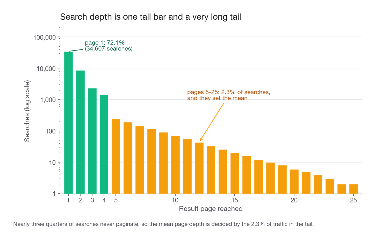
Kyoto, Japan 8569 0.8666 1.1593 0.1024 0.0217 0.9294All five agree on the ordering, which is reassuring and, as we will see, misleading. On the face of it Reykjavik is the problem: fewer than half its searches end on page 1 against 87 percent in Kyoto, and almost 30 percent reach page 3 or deeper, thirteen times the Kyoto rate. The distribution overall is steep: 72.1 percent of searches stop at page 1, 17.8 percent reach page 2, and 2.3 percent go to page 5 or beyond with a maximum of 25. That shape is why the mean is a poor headline. The right tail is 2 percent of traffic and it drags the average around.
Put an interval on the number
Reykjavik has 4,347 searches against Lisbon's 14,834. Any ranking that ignores that is a ranking you cannot defend. Wilson intervals on a proportion are two lines and they cost nothing.
z = 1.96
n, p = metrics["searches"], metrics["page1_rate"]
denom = 1 + z**2 / n
centre = (p + z**2 / (2 * n)) / denom
halfwidth = z * np.sqrt(p * (1 - p) / n + z**2 / (4 * n**2)) / denom
metrics["lo"], metrics["hi"] = centre - halfwidth, centre + halfwidth
print(metrics[["searches", "page1_rate", "lo", "hi"]].round(4).to_string())
searches page1_rate lo hi
Reykjavik, Iceland 4347 0.4619 0.4471 0.4768
Medellin, Colombia 7285 0.5573 0.5459 0.5687
Austin, Texas, United States 12965 0.7168 0.7090 0.7245
Lisbon, Portugal 14834 0.7972 0.7906 0.8035
Kyoto, Japan 8569 0.8666 0.8592 0.8736The intervals are narrow and none overlap, so the ordering is not a sampling artifact. Say so explicitly, and say what would have changed your mind: at 100 searches instead of 4,347, Reykjavik's interval would span roughly 0.37 to 0.56, overlap Medellin's 0.546 to 0.569, and force you to report a tie. Note how much shrinkage that takes. At 300 searches the interval only widens to 0.41 to 0.52, still clearing Medellin's lower bound by almost three points, and the two do not touch until Reykjavik is down near 135 searches. Compute that crossover rather than eyeballing it. The instinct that a small sample automatically buys a tie is off by a factor of three here, and an interviewer doing the arithmetic in their head will catch it.
Interview tip: Any per-group rate you rank on needs an interval and a minimum-volume rule stated up front. "I excluded cities under 500 searches" is a sentence that buys you credibility for free.
Step 5: the ranking is confounded, and you can show it
Where the confound comes from
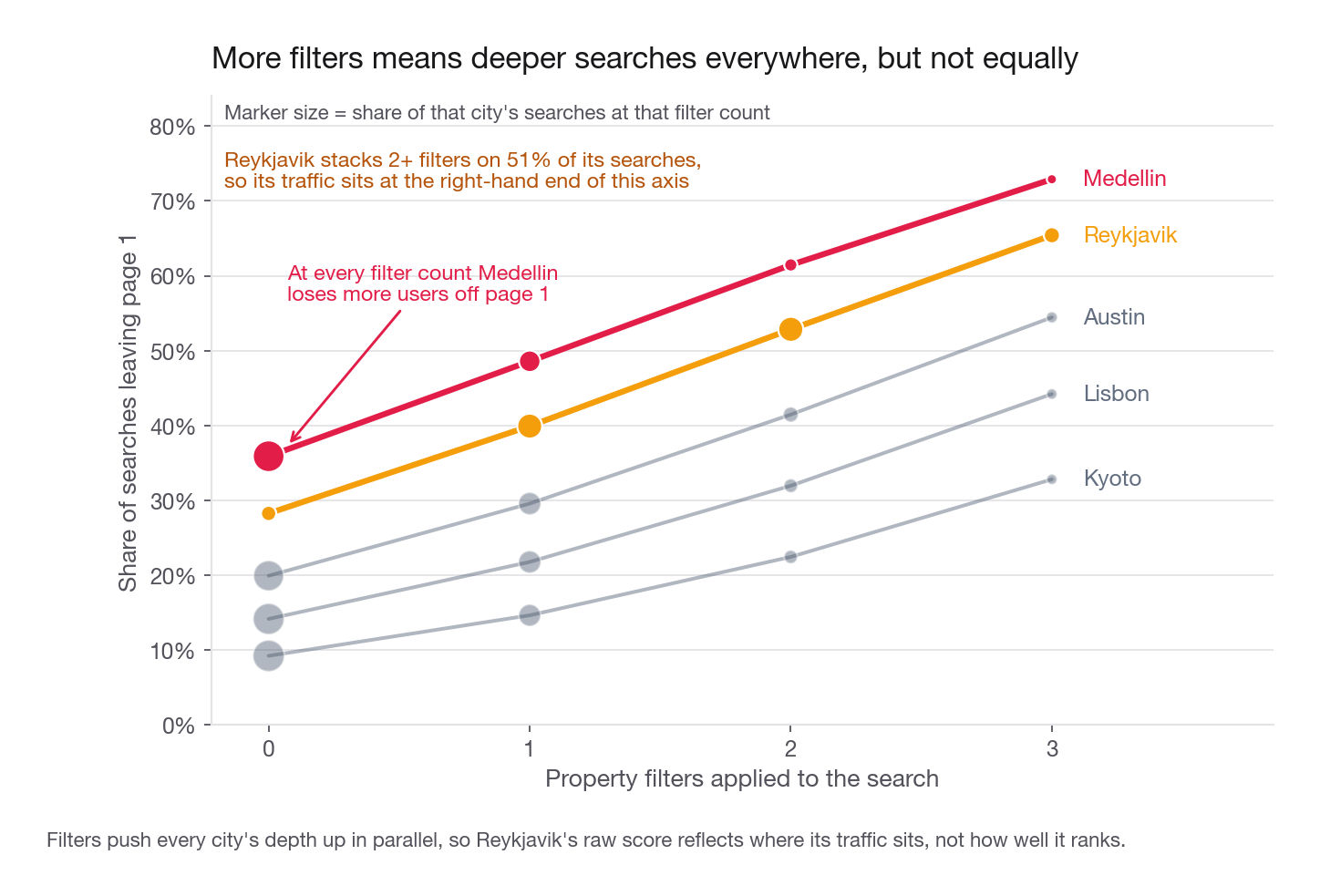
Depth is not only a property of the ranker. It is also a property of the question. A user who applies three filters has told the engine to shrink the candidate set, and a shrunken set paginates sooner. A party of eight is searching a much thinner slice of inventory than a couple. Both of those raise page depth without the ranking model being any worse.
So before crediting or blaming a city, look at what its users are asking for.
wide["big_party"] = wide["party"] >= 6
wide["long_stay"] = wide["nights"] >= 7
mix = wide.groupby("city").agg(searches=("page", "size"),
                               mean_filters=("n_filters", "mean"),
                               share_2plus=("n_filters", lambda s: (s > 1).mean()),
                               mean_party=("party", "mean"),
                               share_big=("big_party", "mean"))
print(mix.round(3).to_string())| City | Searches | Mean filters | Share with 2+ filters | Mean party | Share party 6+ |
|---|---|---|---|---|---|
| Austin, Texas, United States | 12,965 | 0.614 | 14.3% | 3.52 | 10.5% |
| Kyoto, Japan | 8,569 | 0.506 | 10.1% | 3.01 | 6.5% |
| Lisbon, Portugal | 14,834 | 0.535 | 10.9% | 3.55 | 11.2% |
| Medellin, Colombia | 7,285 | 0.489 | 9.8% | 3.05 | 7.3% |
| Reykjavik, Iceland | 4,347 | 1.527 | 51.0% | 6.56 | 69.1% |
There it is. Reykjavik is not a normal city here. Half its searches stack two or more filters against roughly 10 percent elsewhere, and 69 percent of its parties have six or more people against 6 to 11 percent elsewhere. Roamly's Iceland traffic is group trips: a lodge for eight, with parking and a washer, over a long weekend. Those run deep against any ranker.
Medellin, by contrast, has the lightest filter usage of all five cities and small parties, and it still sends 44 percent of its searches past page 1. That is a much more damning number than it first appeared.
Direct standardization
The fix is to compare cities at the same query mix. Cut the data into strata defined by the things that drive depth for non-ranking reasons, compute the page-1 rate inside each stratum, and then reweight every city to the overall mix.
wide["p1"] = wide["page"] == 1
strata = ["n_filters", "big_party", "long_stay"]
w_all = wide.groupby(strata).size() / len(wide)
cells = wide.groupby(["city"] + strata)["p1"].agg(["mean", "size"])

adjusted = {}
for city_name, sub in cells.groupby(level=0):
    s = sub.droplevel(0)
    w = w_all.reindex(s.index).fillna(0)
    ok = s["size"] >= 30                       # ignore cells too thin to estimate
    adjusted[city_name] = float((s["mean"][ok] * w[ok]).sum() / w[ok].sum())

print(pd.Series(adjusted).sort_values().round(4).to_string())
Medellin, Colombia 0.5409
Reykjavik, Iceland 0.6135
Austin, Texas, United States 0.7149
Lisbon, Portugal 0.7889
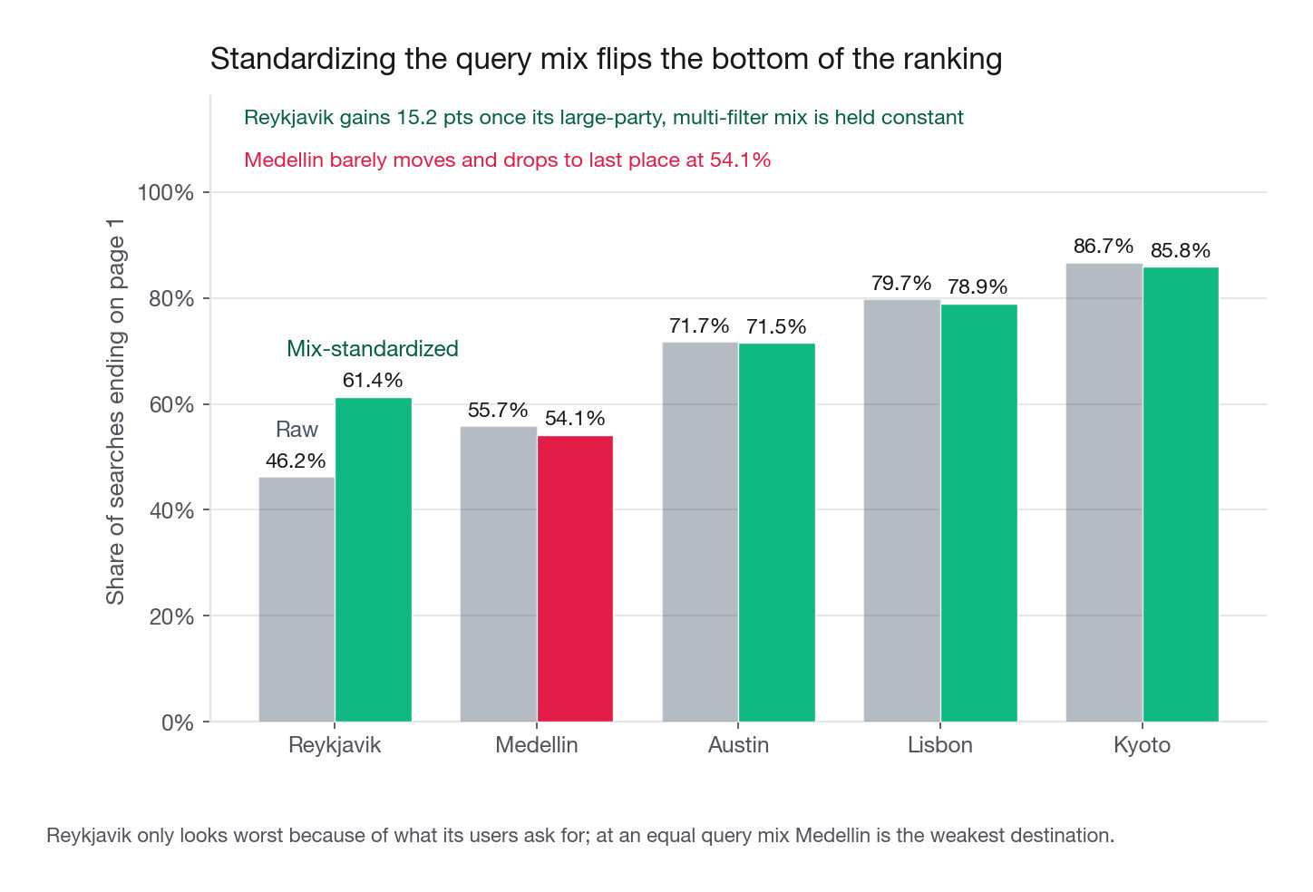
Kyoto, Japan 0.8583The ranking flips at the top. Reykjavik moves from 0.462 to 0.614 once you compare it against other three-filter, eight-guest, seven-night searches, while Medellin barely moves and lands last at 0.541. Austin, Lisbon and Kyoto shift by less than one point because their mixes were already close to the population average.
There are 80 city-by-stratum cells and 70 clear the 30-search floor. Dropping thin cells and renormalizing the weights keeps a single 4-search cell from swinging a city, and it is also why the stable cities move slightly rather than not at all. State that floor in the write-up.
The same answer as a regression
Standardization is transparent but it burns cells fast as you add covariates. A logistic model with city indicators does the same job and scales better.
import statsmodels.formula.api as smf

wide["deep"] = (wide["page"] > 1).astype(int)
model = smf.logit("deep ~ C(city, Treatment('Kyoto, Japan'))"
                  " + n_filters + big_party + long_stay", data=wide).fit(disp=0)
coef = model.summary2().tables[1][["Coef.", "Std.Err."]]
coef["odds_ratio"] = np.exp(coef["Coef."])
coef.index = [i.replace("C(city, Treatment('Kyoto, Japan'))[T.", "city[T.")
               .replace("United States", "US") for i in coef.index]
print(coef.round(3).to_string())
Coef. Std.Err. odds_ratio
Intercept -2.286 0.035 0.102
city[T.Austin, Texas, US] 0.895 0.038 2.449
city[T.Lisbon, Portugal] 0.484 0.038 1.623
city[T.Medellin, Colombia] 1.706 0.040 5.509
city[T.Reykjavik, Iceland] 1.354 0.050 3.872
big_party[T.True] 0.329 0.033 1.390
long_stay[T.True] 0.204 0.023 1.226
n_filters 0.523 0.013 1.688Read the covariates first, because they are the mechanism. Each extra filter multiplies the odds of leaving page 1 by 1.69, a party of six or more by 1.39, a stay of a week or longer by 1.23. Those are large, and they are properties of the query, not the ranker. Now the city effects, all relative to Kyoto: Medellin at 5.51 times the odds of a deep search, Reykjavik at 3.87. Same conclusion as standardization by a different route, and that agreement is worth one sentence in the write-up.
What to write down
The finished answer is not "Medellin". It is roughly this.
Raw depth data names Reykjavik as the weakest destination, with 46.2 percent of searches ending on page 1 against a 72.1 percent platform average. That reading is wrong. Reykjavik's traffic is overwhelmingly large-group, multi-filter searches, 69 percent of its parties are six or more against 6 to 11 percent everywhere else, and both attributes raise page depth independently of ranking quality. Standardizing all five cities to the platform's query mix moves Reykjavik to 61.4 percent and leaves Medellin last at 54.1 percent, and a logistic model with city fixed effects agrees, putting Medellin at 5.51 times Kyoto's odds of a deep search versus Reykjavik's 3.87. Recommendation: point the ranking team at Medellin, and put Reykjavik second rather than clearing it. Its deficit does not disappear under adjustment: 61.4 percent standardized still trails Austin by ten points, and restricting to exactly the searches the mix story blames, party of six or more carrying two or more filters, Reykjavik lands on page 1 only 33.1 percent of the time on 1,540 searches against Austin's 41.2 and Lisbon's 51.6. Compared like for like it is still the second weakest destination. City fixed effects absorb ranking quality and inventory depth in one term, so this file cannot say which of the two is driving that residual. Ask for listing counts per city and results per page, then rerun the comparison.
The discipline in that last move is the part worth copying. The tempting version says Reykjavik's leftover gap is a supply problem, which sounds sophisticated and closes the story neatly. It is also untestable with what you were given: inventory is not in this file, it is the first item in the blind-spot list below, and the residual you would be dissolving sits more than ten standard errors from zero. Handing a large unexplained effect to an unobservable cause is the move interviewers downgrade hardest, because it is indistinguishable from wanting the tidy answer. Name the alternative, name the column that would settle it, and leave it open.
That paragraph is the submission. Everything above it is the evidence.
Interview tip: When an adjustment flips your answer, lead with the flip. "The obvious ranking is wrong and here is why" is the strongest opening sentence a take-home write-up can have.
What this metric still cannot see
Naming the blind spots unprompted is what separates a senior answer from a correct one. Five that matter here.
Inventory size is invisible. A city with 40 listings cannot generate a page 3, so it will score beautifully on any depth metric while offering users almost nothing. Kyoto's 86.7 percent could be excellent ranking or a thin catalog, and this file cannot tell you which. Ask for listing counts per city and results per page.
Abandonment is invisible. A user who searches, sees nothing usable, and closes the tab looks identical to a user who found the perfect place in slot two. Both stop on page 1. That is the fundamental weakness of a depth-only metric and it is the reason it must be paired with a booking or contact rate as a guardrail. Improving page-1 share while bookings fall is a regression dressed as a win.
Intent is invisible. Some people paginate because they enjoy browsing, especially early in trip planning. Lead time, checkin minus the search date, is a decent proxy and belongs in the model if you are given a search timestamp.
Page size is a hidden lever. Showing 40 results per page instead of 20 halves the page-2 rate without improving relevance at all. Confirm the page size is constant across cities before comparing them, otherwise you are measuring a front-end config.
Bots and scrapers live in the tail. The 25-page search is more likely a crawler than a traveler. Cap depth at a high percentile or filter by user agent before shipping, and report how much the ranking moves when you do.
The warehouse version
Once the long table lands in a database, both metrics are ordinary SQL, and this is the form the data engineer will ask for.
WITH parsed AS (
  SELECT search_id,
         MAX(value) FILTER (WHERE param = 'city')                 AS city,
         MAX(value) FILTER (WHERE param = 'result_page')::int     AS result_page,
         COUNT(*)   FILTER (WHERE param = 'features')             AS n_filters
  FROM search_param
  GROUP BY search_id
)
SELECT city,
       COUNT(*)                                   AS searches,
       ROUND(AVG((result_page = 1)::int), 4)      AS page1_rate,
       ROUND(AVG(LN(result_page))::numeric, 4)    AS mean_log_depth,
       ROUND(AVG((result_page >= 3)::int), 4)     AS deep3_rate
FROM parsed
GROUP BY city
HAVING COUNT(*) >= 500
ORDER BY page1_rate;
Run against PostgreSQL 16 on the 317,653-row long table, that returns the metrics table from step four to the digit.
             city             | searches | page1_rate | mean_log_depth | deep3_rate
------------------------------+----------+------------+----------------+------------
 Reykjavik, Iceland           |     4347 |     0.4619 |         0.5974 |     0.2965
 Medellin, Colombia           |     7285 |     0.5573 |         0.4444 |     0.2071
 Austin, Texas, United States |    12965 |     0.7168 |         0.2471 |     0.0916
 Lisbon, Portugal             |    14834 |     0.7972 |         0.1633 |     0.0448
 Kyoto, Japan                 |     8569 |     0.8666 |         0.1024 |     0.0217
That ::numeric is not decoration, and the reason is worth knowing before you type SQL in front of someone. PostgreSQL ships three round signatures and only one of them takes a precision argument: round(numeric, integer). LN returns double precision, so AVG(LN(result_page)) is double precision and ROUND(AVG(LN(result_page)), 4) dies with function round(double precision, integer) does not exist. The ROUND(..., 4) on the two rate columns survives untouched because AVG over an integer returns numeric. That asymmetry, the same wrapper working on two columns and failing on a third, is the fingerprint of a query nobody ran. Cast to numeric before rounding, and execute it before you paste it into a write-up.
The standardized version is the same aggregate run twice, at city-by-stratum grain and at stratum grain, then joined.
WITH cells AS (
  SELECT city, n_filters, big_party,
         AVG((result_page = 1)::int) AS p1, COUNT(*) AS n
  FROM search_features GROUP BY 1, 2, 3
), weights AS (
  SELECT n_filters, big_party, COUNT(*) AS w
  FROM search_features GROUP BY 1, 2
)
SELECT c.city,
       ROUND(SUM(c.p1 * w.w) / SUM(w.w), 4) AS standardized_page1_rate
FROM cells c JOIN weights w USING (n_filters, big_party)
WHERE c.n >= 30
GROUP BY c.city
ORDER BY standardized_page1_rate;
city | standardized_page1_rate
------------------------------+-------------------------
Medellin, Colombia | 0.5388
Reykjavik, Iceland | 0.6135
Austin, Texas, United States | 0.7100
Lisbon, Portugal | 0.7889
Kyoto, Japan | 0.8574The same COUNT(*)::float habit would have broken this one too: float times numeric is float, and the division lands back in the two-argument round that does not exist. Dropping the cast leaves w a bigint and p1 a numeric, so the product, both sums, and the quotient are all numeric and the round resolves. Note also that this query strata on two variables where the Python used three, so the numbers land a hair off: Medellin 0.5388 against 0.5409, Austin 0.7100 against 0.7149, same ordering. Add long_stay to both GROUP BY lists and the join key to make them agree exactly, and say which version you ran.
The HAVING COUNT(*) >= 500 and WHERE c.n >= 30 clauses are the minimum-volume rules from earlier, written into the query so nobody has to remember them.
Common traps
Building a key-to-value dictionary. Repeated stay.features keys collapse to one and the multi-filter count silently becomes zero. Fix: parse_qsl, which returns pairs, and keep a long table so repeats are rows.
Splitting on = with str.split("="). Any value containing an unescaped =, base64 tokens especially, produces more than two pieces and either crashes or truncates. Fix: let the library split on the first delimiter only.
Forgetting to decode. Lisbon%2C+Portugal and Lisbon, Portugal group as different cities, so one destination appears twice with half the volume each. Fix: decode at parse time, before anything is grouped.
Dropping blank values. parse_qsl discards stay.instantBook= unless you pass keep_blank_values=True, erasing the difference between cleared and never-shown. Fix: pass the flag, always.
Imputing zero for absent numeric filters. Absent stay.priceCeiling means no cap, not a cap of zero, and a mean over the imputed column is nonsense. Fix: zero-fill counts and checkboxes only, leave numeric filters missing.
Assuming positional columns. Optional parameters appear in arbitrary order, so the third field is not reliably anything. Fix: never index by position, and never assume the parameter list from a sample of one URL.
Using mean page depth as the headline. It is dominated by a 2 percent tail and it prices a page 9 to 8 move the same as a page 2 to 1 move. Fix: lead with the page-1 share, keep the mean of the log as a sensitivity check.
Ranking cities without intervals or a volume floor. A small city can top or bottom a leaderboard on noise alone. Fix: Wilson intervals, a stated minimum, and an explicit "these two are tied" when they overlap.
Ranking on a raw rate when the query mix differs. This is the big one and it flipped the answer here. Fix: standardize to a common mix or fit city fixed effects with covariates for filter count, party size, and stay length.
Reporting depth alone. A ranker that returns nothing usable produces perfect page-1 rates. Fix: name a booking-side guardrail even if the data to compute it was not provided.
Skipping the grain check. If a row were a page view rather than a search, every number on this page would be wrong. Fix: run the fingerprint diagnostic and report what it found.
Quick self-check
Answer these out loud before you consider the challenge finished.
A colleague parses the URLs with
dict(pair.split("=") for pair in query.split("&"))and reports that no search ever used more than one property filter. Name the two independent defects in that line and the one function call that fixes both.stay.kidsis absent on 73 percent of rows andstay.priceCeilingis absent on 78 percent. Explain why one of those should become zero and the other should stay missing, and describe the specific wrong conclusion that follows from getting it backwards.You have to choose one headline number for a quarterly ranking goal. Defend the share of searches ending on page 1 against the mean of the log of page depth, in terms of what each one rewards the team for doing.
Reykjavik's raw page-1 rate is 0.462 and its standardized rate is 0.614. Explain in two sentences what standardization did, and say what you would need to see in the mix table for standardization to be unnecessary.
Kyoto scores best on every depth metric. Give two distinct explanations for that, one flattering to the ranking team and one not, and say what single extra column would let you tell them apart.
Your recommendation is to prioritize Medellin. The head of product asks how you would know in six weeks whether the ranking work paid off. Name the primary metric, the guardrail, and the reason a page-1 improvement with flat bookings should not be shipped.
If question 4 or 6 feels shaky, reread step five. Everything else here is craft, and craft can be learned in an afternoon. The mix argument is the part that gets you to the onsite.