3.3 Challenge: Org Hierarchy, Levels, and Pay Equity
Find the core decision, design, or behavior signal.
Turn the lesson into a concise response blueprint.
Name the trap you would avoid in a real interview.
Use these checkpoints as your reading path before diving into the full lesson.
- 1What this lesson is for
- 2The brief and the two tables
- 3The integrity pass, before anything else
- 4Part 1: turning an edge list into levels
- 5Two definitions that agree on paper and...
Two files land in your inbox on a Friday. One holds 7,954 rows of employee ids paired with manager ids. The other holds salaries. The brief asks you to assign everyone an organisational level, work out how many people each manager is ultimately responsible for, model salary, and then tell the Head of People whether Vantage Software pays its staff fairly. The first two tasks are graph problems with one correct answer and three tempting wrong ones. The third is routine. The fourth is where the grade is decided, because the same regression supports two opposite conclusions depending on one variable you either include or leave out, and most candidates never notice they made a choice at all.
What this lesson is for
This challenge tests three separate skills and reviewers score them separately.
The first is whether you can turn an edge list into a hierarchy without hand-waving. There is no level column anywhere in the data. You have to derive it, and the derivation has a subtlety that a balanced org chart hides and a real one exposes.
The second is whether you can accumulate a quantity up a tree. Total span of control is not a groupby. It is a recursion, and there are two clean ways to write it plus one popular way that silently undercounts.
The third, and the one that separates offers from rejections, is whether you know what the coefficient on a sensitive attribute means once controls arrive. Put level in the model and the gender coefficient collapses from roughly 15 percent to under 2. Leave it out and it stays large. Both models are correctly fit, they answer different questions, and only one answers what the Head of People asked.
Interview tip: When a reviewer asks "did you control for level?", the right first move is to ask what decision the answer feeds, not to say yes or no.
The brief and the two tables
Vantage Software is a fictional 7,954 person enterprise software company. You are given two extracts from the human resources system.
| Table | Column | Meaning |
|---|---|---|
org | employee_id | Unique person key |
org | manager_id | The employee_id this person reports to, -1 for the chief executive |
org | dept | One of platform, revenue, growth, people_ops, or exec |
people | employee_id | Joins to org.employee_id |
people | gender | Recorded as F or M in this extract |
people | age_band | under_40 or 40_plus |
people | degree | high_school, bachelor, master, phd |
people | yrs_experience | Total prior work experience in years |
people | signing_bonus | 1 if a signing bonus was paid at hire |
people | salary | Current annual base pay in dollars |
Vantage runs six bands defined by management responsibility rather than title: L1 manages nobody, L2 is the direct manager of L1 staff, L3 manages L2 staff, and so on up to L6, the chief executive. Note that the definition points downward, from a person to the people below them. That matters in about four hundred words.
Three things the brief omits, and all three change your answer:
Whether every
manager_idresolves to a real employee. It does not.Whether the reporting graph is a tree. It is not.
Whether
salaryis base pay, total cash, or something typed by hand. Nine rows suggest the last.
This block builds both tables deterministically. Every figure quoted for the rest of the lesson comes out of it, including the defects, which were planted because real human resources extracts have them.
import numpy as np
import pandas as pd

SEED = 4407
rng = np.random.default_rng(SEED)
FAN = [6, 4, 5, 6, 8]
PAT = ["platform"] * 4 + ["revenue"] * 3 + ["growth"] * 2 + ["people_ops"]
rows, nxt, j = [(1, -1, 6, "exec")], 2, 0
for step, fan in enumerate(FAN):
    band = 5 - step
    for p in [r for r in rows if r[2] == band + 1]:
        for _ in range(max(2, fan + int(rng.integers(-1, 2)))):
            dept = PAT[j % 10] if band == 4 else p[3]
            j += band == 4
            rows.append((nxt, p[0], band, dept))
            nxt += 1
tree = pd.DataFrame(rows, columns=["employee_id", "manager_id", "band", "dept"])
flat = rng.choice(tree.index[tree.band == 1].to_numpy(), 340, replace=False)
tree.loc[flat, "manager_id"] = rng.choice(tree.employee_id[tree.band.isin([3, 4])].to_numpy(), 340)
n, b = len(tree), tree.band.to_numpy()
AF = {"platform": -0.75, "revenue": -0.25, "growth": 0.35, "people_ops": 1.10, "exec": -0.70}
DS = {"platform": 0.20, "revenue": 0.05, "growth": -0.04, "people_ops": -0.30, "exec": 0.0}
DG = {"high_school": 0.0, "bachelor": 0.03, "master": 0.05, "phd": 0.07}
w = rng.random(n) < 1 / (1 + np.exp(-(tree.dept.map(AF).to_numpy() - 0.95 * (b - 1))))
yrs = np.clip(np.round((np.array([1, 3, 5, 7, 9, 26])[b - 1] + rng.gamma(2.4, 2.1, n)) * (1 - .06 * w)), 1, 38)
deg = rng.choice(list(DG), n, p=[.08, .44, .34, .14])
bonus = (rng.random(n) < 0.30).astype(int)
z = (np.log(122000) + np.array([0, .42, .80, 1.14, 1.42, 2.00])[b - 1] + tree.dept.map(DS).to_numpy()
     + 0.017 * np.minimum(yrs, 20) + pd.Series(deg).map(DG).to_numpy() + 0.02 * bonus
     - 0.043 * w * (tree.dept == "revenue").to_numpy() + rng.normal(0, 0.18, n))
people = pd.DataFrame({"employee_id": tree.employee_id, "gender": np.where(w, "F", "M"),
    "age_band": np.where(rng.random(n) < 1 / (1 + np.exp(-(-2.6 + .20 * yrs))), "40_plus", "under_40"),
    "degree": deg, "yrs_experience": yrs.astype(int), "signing_bonus": bonus,
    "salary": np.round(np.exp(z) / 500) * 500})
people.loc[rng.choice(n, 9, replace=False), "salary"] /= 1000
people.loc[rng.choice(n, 96, replace=False), "salary"] = np.nan
people = pd.concat([people, people.sample(23, random_state=7)], ignore_index=True)
tree.loc[tree.employee_id == 4210, "manager_id"] = 99999
tree.loc[tree.employee_id.isin([6033, 6034]), "manager_id"] = [6034, 6033]
org = tree[["employee_id", "manager_id", "dept"]].copy()
The generator keeps a band column for its own bookkeeping. The delivered org table does not have it, which is the whole point of the first task.
The integrity pass, before anything else
Four checks, ninety seconds, an hour saved later.
ids = set(org.employee_id)
print("org rows", len(org), "people rows", len(people))
print("duplicate people ids", people.employee_id.duplicated().sum())
print("null salary", people.salary.isna().sum())
print("salary below 10k", (people.salary < 10000).sum())
print("roots", (org.manager_id == -1).sum())
print("unresolved manager ids", (~org.manager_id.isin(ids) & (org.manager_id != -1)).sum())
print("self managers", (org.employee_id == org.manager_id).sum())
org rows 7954 people rows 7977
duplicate people ids 23
null salary 97
salary below 10k 9
roots 1
unresolved manager ids 1
self managers 0Twenty-three employees appear twice in people, so a join before deduplication gives them double weight in every mean and quietly makes your model table 7,977 rows. Ninety-seven salaries are missing. Nine sit under 10,000 and read 113, 163.5, 168, 170.5, 181, 186.5, 193, 211, and 247.5, which are annual salaries typed in thousands. Multiplying by 1,000 lands each inside the plausible range for its band, so repair them rather than dropping them, and say so in the report.
The root carries -1, not a null. A candidate who writes org.manager_id.isnull() to find the chief executive finds nobody, starts with an empty frontier, and produces a level column that is entirely one value. Read the sentinel before trusting a null check.
Interview tip: Say the row counts out loud before and after every join. "7,954 in, 7,977 out, so I have 23 duplicate keys" is the single most reliable way to look experienced in the first five minutes.
Part 1: turning an edge list into levels
Two definitions that agree on paper and disagree in the data
There are two natural ways to number someone's position in a hierarchy.
Depth counts hops downward from the chief executive. The root has depth 0, its reports have depth 1, and so on. It is a breadth-first walk and it is what most candidates write.
Height counts hops upward from the bottom. Anyone with no reports has height 0, anyone whose deepest subordinate chain is one hop long has height 1. It requires processing children before parents.
In a perfectly regular chart where every branch has the same length, level = max_depth - depth + 1 and level = height + 1 agree, so nobody notices. Vantage is not regular. Some individual contributors report straight to an L3 or an L4, which is ordinary in a real company and fatal to the depth version.
Here is depth, which you need anyway.
kids = org[org.manager_id != -1].groupby("manager_id")["employee_id"].apply(list).to_dict()
root = org.loc[org.manager_id == -1, "employee_id"].tolist()

depth, frontier, d = {}, root, 0
while frontier:
    for e in frontier:
        depth[e] = d
    frontier = [c for e in frontier for c in kids.get(e, [])]
    d += 1

print("reached", len(depth), "of", len(org), "max depth", max(depth.values()))
print(pd.Series(depth).value_counts().sort_index().to_dict())
reached 7951 of 7954 max depth 5
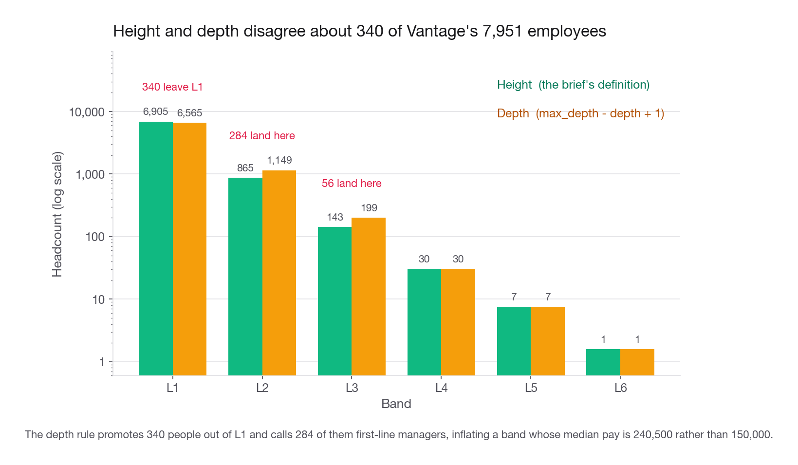
{0: 1, 1: 7, 2: 30, 3: 199, 4: 1149, 5: 6565}Now height, computed by walking the nodes in order of decreasing depth so that every child is finished before its parent is touched. That ordering is the trick, and it removes any need for recursion limits.
order = sorted(depth, key=lambda e: -depth[e])
height = {}
for e in order:
    ch = [c for c in kids.get(e, []) if c in depth]
    height[e] = 0 if not ch else 1 + max(height[c] for c in ch)

lvl = pd.Series(height) + 1
print(lvl.value_counts().sort_index().to_dict())
{1: 6905, 2: 865, 3: 143, 4: 30, 5: 7, 6: 1}The two answers are not the same, and the disagreement is not a rounding artefact.
| Band | From height, the brief's definition | From depth | Difference |
|---|---|---|---|
| L1 | 6,905 | 6,565 | 340 people |
| L2 | 865 | 1,149 | 284 people |
| L3 | 143 | 199 | 56 people |
| L4 | 30 | 30 | 0 |
| L5 | 7 | 7 | 0 |
| L6 | 1 | 1 | 0 |
Exactly 340 people are labelled managers by the depth rule and manage nobody: 284 sit one hop below an L3 and 56 one hop below an L4. They are senior individual contributors reporting into a second- or third-line manager. Calling them first-line managers inflates the management population by a third and puts 340 non-managers into the band whose median pay is 240,500 rather than 150,000.
The brief defines a band by who you manage, which is a height definition, so height wins. Keep depth as a second column named reporting_depth, since it is useful for escalation paths, and say in the write-up that you computed both and that they disagree for 340 people. That sentence is worth more than the rest of the section.
The graph is not a tree until you prove it is
The breadth-first walk reached 7,951 of 7,954 people. Three are unreachable, and they are unreachable for two different reasons.
unreached = sorted(set(org.employee_id) - set(depth))
print("unreachable", unreached)
print(org[org.employee_id.isin(unreached)].to_string(index=False))
unreachable [4210, 6033, 6034]
employee_id manager_id dept
4210 99999 platform
6033 6034 platform
6034 6033 platformEmployee 4210 points at manager 99999, who does not exist. That is a dangling foreign key, probably a manager who left and whose reports were never reassigned. Employees 6033 and 6034 are listed as each other's manager, which is a two-node cycle. A naive recursive walk on that pair loops until the interpreter gives up.
Two habits follow. Terminate every traversal on the frontier going empty rather than at a fixed depth, and track a visited set so a cycle cannot re-enter. Then compare reachable count against table length, every time.
Do not drop the three silently. Say: three employees, 0.04 percent of headcount, cannot be placed, one because their manager id resolves to nobody and two because of a circular record, all three are excluded from level and span, and here are the ids so the system can be fixed.
Interview tip: "I found a two-node cycle in the reporting graph" is a sentence that ends the technical portion of the interview in your favour, because it proves you validated rather than assumed.
The same thing in SQL
Warehouses handle this with a recursive common table expression, and interviewers ask for it often enough that you should be able to write it from memory. The cycle guard is the part people forget.
WITH RECURSIVE walk AS (
    SELECT employee_id,
           0 AS reporting_depth,
           ARRAY[employee_id] AS seen
    FROM org
    WHERE manager_id = -1
    UNION ALL
    SELECT o.employee_id,
           w.reporting_depth + 1,
           w.seen || o.employee_id
    FROM org o
    JOIN walk w ON o.manager_id = w.employee_id
    WHERE NOT o.employee_id = ANY(w.seen)
)
SELECT employee_id, reporting_depth FROM walk;
Height needs the opposite direction, so either run a second recursion from the leaves or accept depth in the warehouse and apply the height correction in the analytical layer. Say which you would do and why rather than pretending SQL makes it free.
Part 2: total span of control
Direct reports is a value_counts on manager_id. Total span is every person underneath you at any distance, which needs accumulation up the tree.
State the convention before you compute: if an L3 has 8 direct reports and each manages 7 people, their total span is 8 plus 56, which is 64, and it excludes themselves. Write that arithmetic down, because the reading where a manager counts their own head shifts every number by one and reviewers do check.
The clean implementation reuses the ordering you already built for height. Process deepest first, and by the time you reach a node, every child already carries its own total.
span = {}
for e in order:
    ch = [c for c in kids.get(e, []) if c in depth]
    span[e] = len(ch) + sum(span[c] for c in ch)

nodes = pd.DataFrame({
    "employee_id": list(depth),
    "level": [height[e] + 1 for e in depth],
    "reporting_depth": [depth[e] for e in depth],
    "direct_reports": [len([c for c in kids.get(e, []) if c in depth]) for e in depth],
    "total_span": [span[e] for e in depth],
}).merge(org[["employee_id", "dept"]], on="employee_id")
Two identities let you prove the result rather than eyeball it, and both are one line.
root_id = root[0]
print("root span", span[root_id], "reachable minus one", len(depth) - 1)
print("sum of spans", nodes.total_span.sum(), "sum of depths", nodes.reporting_depth.sum())
root span 7950 reachable minus one 7950
sum of spans 38085 sum of depths 38085The first is obvious: the chief executive manages everyone reachable except themselves. The second is worth understanding, because it is a free correctness check on any tree accumulation you ever write. Each employee is counted once in the span of every one of their ancestors, and a person's ancestor count is exactly their depth, so the two sums count the same pairs from opposite ends. If they disagree, you have double counting, found in one line rather than in code review.
| Band | People | Median direct reports | Median total span | Mean total span | Largest total span |
|---|---|---|---|---|---|
| L1 | 6,905 | 0 | 0 | 0.0 | 0 |
| L2 | 865 | 8 | 8 | 7.6 | 9 |
| L3 | 143 | 8 | 54 | 53.9 | 70 |
| L4 | 30 | 6 | 238 | 263.8 | 359 |
| L5 | 7 | 4 | 1,213 | 1,134.7 | 1,374 |
| L6 | 1 | 7 | 7,950 | 7,950.0 | 7,950 |
The shape matters. Direct reports barely move across bands, sitting between 4 and 8 the whole way up, while total span multiplies by roughly seven per band. Direct report count is therefore almost useless as a seniority feature while total span is nearly a perfect proxy for band. Hold that thought for the modelling section.
Part 3: the pay question, which is the real challenge
Join the tables, clean what the integrity pass found, and build the analysis frame. Excluding the eight people in the exec department is a judgement call you should state: they have no departmental comparison group, and one of them earns 1,386,500, which drags any mean you compute.
p = people.drop_duplicates("employee_id").copy()
p.loc[p.salary < 10000, "salary"] *= 1000
p = p.dropna(subset=["salary"])

d = nodes.merge(p, on="employee_id")
d["log_salary"] = np.log(d.salary)
d["is_w"] = (d.gender == "F").astype(int)
d["is_manager"] = (d.level >= 2).astype(int)
core = d[d.dept != "exec"].copy()
print(len(d), len(core), core.is_w.sum(), (1 - core.is_w).sum())
7855 7847 3259 4588Report the unadjusted gap first, and label it honestly
Print it from core, which already excludes exec.
print(core.groupby("gender").salary.agg(["size", "mean", "median"])) size mean median
gender
F 3259 151813.746548 144500.0
M 4588 180475.479512 165500.0Women at Vantage average 151,814 against 180,475 for men, a shortfall of 15.9 percent on the mean and 12.7 percent on the median. On logs, which is the scale you should model, the raw gap is 0.1587, or 14.7 percent, with a confidence interval of 13.5 to 15.8 percent.
Publish it. It is also not evidence of anything on its own, and the sentence you attach decides whether the reviewer trusts you. The unadjusted gap answers what the average woman takes home relative to the average man. That is the number most pay-gap reporting regimes require, and it is a composition statistic: it confounds pay-setting with hiring, department mix, and promotion.
Build a ladder of models, not one model
Fit the same specification repeatedly, adding one block of controls at a time, and read the movement rather than the endpoint.
import statsmodels.formula.api as smf

specs = {
    "M1 gender only": "log_salary ~ is_w",
    "M2 + department": "log_salary ~ is_w + C(dept)",
    "M3 + experience, degree, bonus": "log_salary ~ is_w + C(dept) + yrs_experience + C(degree) + signing_bonus",
    "M4 + band": "log_salary ~ is_w + C(dept) + yrs_experience + C(degree) + signing_bonus + C(level)",
}
for name, f in specs.items():
    r = smf.ols(f, core).fit()
    lo, hi = r.conf_int().loc["is_w"]
    print(f"{name:32s} {100*(np.exp(r.params['is_w'])-1):+6.2f}%  "
          f"[{100*(np.exp(lo)-1):+.2f}, {100*(np.exp(hi)-1):+.2f}]  R2={r.rsquared:.3f}")
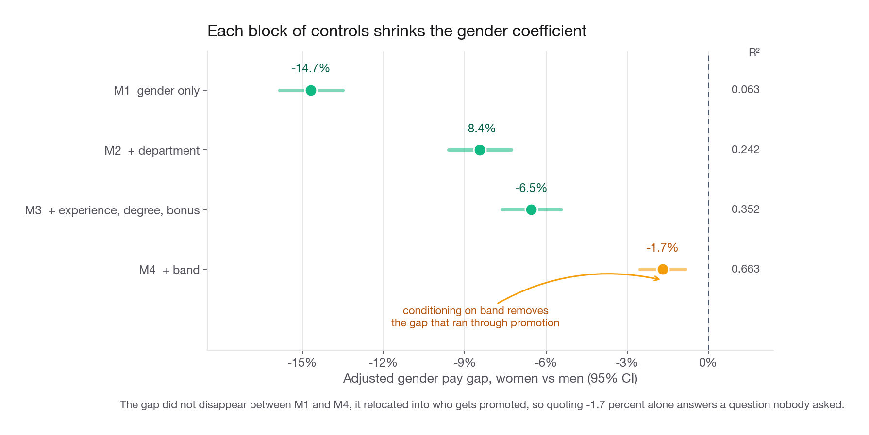
M1 gender only -14.68% [-15.83, -13.51] R2=0.063
M2 + department -8.44% [-9.59, -7.28] R2=0.242
M3 + experience, degree, bonus -6.54% [-7.63, -5.43] R2=0.352
M4 + band -1.69% [-2.53, -0.84] R2=0.663| Specification | Adjusted gap | What it answers |
|---|---|---|
| M1 | -14.7 percent | What the average woman earns relative to the average man |
| M2 | -8.4 percent | The same, comparing within department |
| M3 | -6.5 percent | The same, comparing within department at equal experience and education |
| M4 | -1.7 percent | The same, comparing within department, experience, education, and band |
Two mechanical notes. A coefficient on log salary is only approximately a percentage: exp(-0.1587) - 1 is -14.68 percent while the coefficient reads -15.87, and above about 10 percent a reviewer will notice if you quote the wrong one. And R-squared jumping from 0.352 to 0.663 when band enters is not a sign that band is a better variable, it is a sign that band sits closer to the outcome in the causal chain, which is exactly the problem.
Adding total span on top of band moves the gender coefficient by zero and R-squared by 0.001, which is the span-band collinearity showing up. Do not present both as independent findings.
Why controlling for band hides the thing you were asked to measure
A control variable is appropriate when it is a common cause of both the treatment and the outcome. It is inappropriate, and actively misleading, when it sits on the causal path between them.
Band sits on the path. If promotion decisions at Vantage disadvantage women, then gender causes band, and band causes salary. Conditioning on band asks "among people who reached the same band, is pay equal", which throws away every dollar of the gap that ran through promotion. That is not a technicality here, it is where nearly all of the gap lives.
Test it directly.
lg = smf.logit("is_manager ~ is_w + yrs_experience + C(dept) + C(degree)", core).fit(disp=0)
lo, hi = np.exp(lg.conf_int().loc["is_w"])
print("odds ratio for women", round(np.exp(lg.params["is_w"]), 3), (round(lo, 3), round(hi, 3)))
print("manager rate women", round(core[core.is_w == 1].is_manager.mean(), 4))
print("manager rate men  ", round(core[core.is_w == 0].is_manager.mean(), 4))

women = core[core.is_w == 1].copy()
as_men = women.assign(is_w=0)
print("predicted if promoted like men", round(lg.predict(as_men).mean(), 4))
print("missing women managers", round((lg.predict(as_men).mean() - lg.predict(women).mean()) * len(women)))

lg2 = smf.logit("is_manager ~ is_w + C(dept) + C(degree)", core).fit(disp=0)
print("odds ratio, experience dropped", round(np.exp(lg2.params["is_w"]), 3))
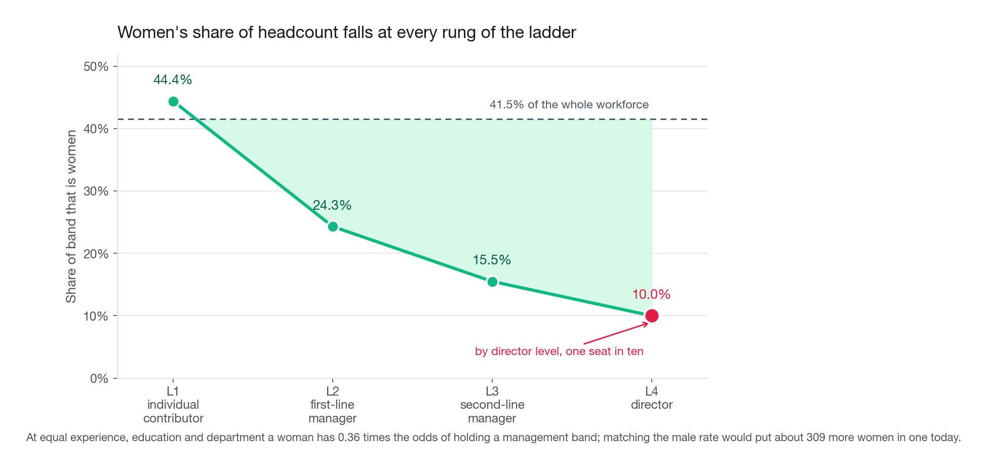
odds ratio for women 0.364 (0.309, 0.429)
manager rate women 0.0715
manager rate men 0.1735
predicted if promoted like men 0.1662
missing women managers 309
odds ratio, experience dropped 0.336At equal experience, equal education, and inside the same department, a woman at Vantage has 0.364 times the odds of holding a management band, with a confidence interval from 0.31 to 0.43. Note the direction: drop yrs_experience and the ratio falls to 0.336, because part of the experience deficit is itself why women are not in management bands. So 0.364 is the conservative reading. Women make up 44.4 percent of L1, 24.3 percent of L2, 15.5 percent of L3, and 10.0 percent of L4. Match the promotion rate and roughly 309 more women would hold a management band today.
So the two headline numbers are not in conflict. The unadjusted gap is 14.7 percent. The within-band gap is 1.7 percent. The difference did not disappear, it relocated into who gets promoted.
The same objection applies to experience
The tempting next move is to call band the one contaminated control and the rest of M3 clean background. Say that and a good reviewer asks why gender cannot cause years of experience. It can: career interruptions, part-time spells, and caregiving accrue before Vantage ever sees you, and not evenly.
gap_raw = smf.ols("yrs_experience ~ is_w", core).fit()
gap_adj = smf.ols("yrs_experience ~ is_w + C(dept) + C(level)", core).fit()
print("raw experience gap   %+.2f yrs  p=%.1e" % (gap_raw.params["is_w"], gap_raw.pvalues["is_w"]))
print("within dept and band %+.2f yrs  p=%.1e" % (gap_adj.params["is_w"], gap_adj.pvalues["is_w"]))

bfml = "log_salary ~ is_w + C(dept)"
for extra in ["", " + yrs_experience", " + C(degree)", " + signing_bonus"]:
    r = smf.ols(bfml + extra, core).fit()
    print("M2%-17s %+6.2f%%" % (extra, 100 * (np.exp(r.params["is_w"]) - 1)))

m2, m2e = smf.ols(bfml, core).fit(), smf.ols(bfml + " + yrs_experience", core).fit()
tot = smf.ols("yrs_experience ~ is_w + C(dept)", core).fit().params["is_w"]
move = 100 * (np.exp(m2e.params["is_w"]) - 1) - 100 * (np.exp(m2.params["is_w"]) - 1)
print("shrinkage %.2f pp = within-band %.2f + band composition %.2f"
      % (move, move * gap_adj.params["is_w"] / tot, move * (tot - gap_adj.params["is_w"]) / tot))
raw experience gap -0.69 yrs p=5.0e-19
within dept and band -0.38 yrs p=1.2e-06
M2 -8.44%
M2 + yrs_experience -6.58%
M2 + C(degree) -8.39%
M2 + signing_bonus -8.47%
shrinkage 1.87 pp = within-band 1.06 + band composition 0.81Women carry 5.85 years of recorded experience against 6.53 for men, and 0.38 of that 0.69 year deficit survives department and band. Experience is a partial mediator too. Conditioning on it answers "among people who arrived with the same experience, is pay fair", which is narrower than what the Head of People asked. Band and experience differ in degree, not in kind.
Experience does all of M3's work: alone it moves the gap from -8.44 to -6.58 percent, while degree lands at -8.39 and signing bonus at -8.47. The M2 to M3 step is one gendered variable, and the last line splits the 1.87 points it absorbs.
Neither piece is neutral. About 1.06 points is women inside a band holding less experience than the men beside them. The other 0.81 runs through band composition: women sit in the lower bands, which hold less experienced people, so part of the move is a back door onto the promotion mediator you just ruled out.
None of that means delete experience. Defend it on decision relevance rather than on a false causal claim: Vantage controls the offer it makes at a given experience level, so holding it fixed produces an actionable number, said in the same breath as the admission that the experience distribution is not gender neutral either.
A formal decomposition makes the same point with one number. Fit the model without gender, predict for everyone, and split the observed gap into the part explained by differences in characteristics and the part that is left over.
| Control set | Explained by characteristics | Left unexplained | Share explained |
|---|---|---|---|
| Department, experience, education, bonus | -0.0965 | -0.0623 | 60.8 percent |
| The same plus band | -0.1434 | -0.0154 | 90.3 percent |
Reading that table as "90 percent is explained, so we are fine" is the most common wrong conclusion on this challenge. Explained means attributable to a measured characteristic, and band is both a measured characteristic and the outcome of a company decision. Explained is not justified.
Interview tip: Present the unadjusted gap, the within-band gap, and the promotion odds ratio as one three-line result, never the middle one alone.
Where the residual gap actually lives
The within-band coefficient of -1.7 percent is statistically significant at this sample size, so do not stop there. Split it.
for dp in ["platform", "revenue", "growth", "people_ops"]:
    s = core[core.dept == dp]
    r = smf.ols("log_salary ~ is_w + yrs_experience + C(degree) + signing_bonus + C(level)", s).fit()
    lo, hi = np.exp(r.conf_int().loc["is_w"]) - 1
    print(f"{dp:11s} n={len(s):5d} {100*(np.exp(r.params['is_w'])-1):+6.2f}%  "
          f"[{100*lo:+.2f}, {100*hi:+.2f}]  p={r.pvalues['is_w']:.3g}")
platform n= 3128 -0.32% [-1.73, +1.11] p=0.66
revenue n= 2325 -5.28% [-6.70, -3.83] p=2.82e-12
growth n= 1677 -0.10% [-1.85, +1.68] p=0.911
people_ops n= 717 +1.59% [-1.34, +4.61] p=0.29Three departments show nothing. Revenue shows 5.28 percent, tightly estimated on 2,325 people. A gender-by-department interaction confirms it: the revenue term is -0.0505 with a p-value of 1.7 times ten to the minus five, and the others are indistinguishable from zero.
That is a finding you can act on, and it converts to money. Revenue employs 914 women whose average salary is 148,895. Closing a 5.28 percent gap for them costs about 7.2 million dollars a year, or roughly 0.54 percent of the 1,322.8 million dollar payroll in scope. Put both the absolute and the relative figure in the memo, because the first sounds enormous and the second sounds manageable, and the second is the honest framing.
Contrast that with a table any candidate could produce and many stop at.
| Band | Median, women | Median, men | Raw gap | Women in band |
|---|---|---|---|---|
| L1 | 141,000 | 157,000 | -10.2 percent | 3,026 |
| L2 | 223,500 | 248,500 | -10.1 percent | 208 |
| L3 | 317,500 | 362,000 | -12.3 percent | 22 |
| L4 | 398,500 | 538,500 | -26.0 percent | 3 |
Every cell shows a double-digit gap, and every cell is misleading. Within L1, women are 15.5 percent of headcount in people_ops against 4.6 percent for men, and people_ops has the lowest pay of any department. Once department and experience are held fixed, the L1 gap in platform and growth is statistically zero. The L4 row rests on three women and belongs in a footnote, not a headline. A within-band median cut is not an adjusted comparison, and presenting it as one is the fastest way to lose a reviewer's trust.
The attribute that looks like a finding and is not
Run the same ladder on age band and watch it evaporate.
| Specification | Effect of 40_plus | p-value |
|---|---|---|
| Age band only | +7.06 percent | 6 times ten to the minus 16 |
| Plus years of experience | -1.34 percent | 0.10 |
| Plus experience, department, band, education | -0.76 percent | 0.14 |
Older employees earn 7 percent more, and the entire effect is experience. Once you hold experience fixed, the coefficient crosses zero and stops being distinguishable from noise. Report it exactly that way. Publishing "no evidence of an age-related pay difference once tenure is accounted for" is a real result, and it also demonstrates that your method is capable of returning a null, which makes the revenue finding more credible rather than less.
Interview tip: Always include one sensitive attribute where your answer is "we looked and found nothing", because a report that finds a problem everywhere it looks reads as motivated.
Why a random forest is the wrong instrument here
The obvious modelling move on a task phrased as "build a model to predict salary" is to throw a random forest at it. Do that if you like, it fits fine, but understand what it can and cannot tell you.
from sklearn.ensemble import RandomForestRegressor
from sklearn.model_selection import train_test_split

X = pd.get_dummies(core[["dept", "degree", "age_band", "gender",
                         "yrs_experience", "signing_bonus", "level", "total_span"]])
Xtr, Xte, ytr, yte = train_test_split(X, core.log_salary, test_size=0.3, random_state=11)
rf = RandomForestRegressor(n_estimators=300, min_samples_leaf=5, random_state=11, n_jobs=-1).fit(Xtr, ytr)
imp = pd.Series(rf.feature_importances_, index=X.columns).sort_values(ascending=False)
print("test R2", round(rf.score(Xte, yte), 3))
print(imp.head(6).round(3).to_dict())
test R2 0.661
{'level': 0.286, 'total_span': 0.262, 'dept_platform': 0.201,
'dept_people_ops': 0.104, 'yrs_experience': 0.075, 'signing_bonus': 0.012}Gender lands at 0.006, near the bottom. Predictions fall within 15 percent of actual pay for 59.1 percent of the test set, which is honest but unremarkable.
Three reasons that ranking cannot answer the question it appears to answer. Impurity importance is diluted across correlated features, and band and total span are nearly the same variable, so together they absorb about 55 percent of the total. Importance has no sign and no interval, so it cannot separate a small effect from none. And band is in the model, so the forest sits in exactly the conditioning position that erases the gender signal by construction.
Use a flexible model for a prediction and a specified linear model on log pay when you need a signed, tested coefficient. Here you need the coefficient, so the regression is the deliverable and the forest is a robustness check at best.
Part 4: what you actually send the Head of People
The memo is the deliverable. Four short paragraphs, in order.
The headline. Women at Vantage earn 14.7 percent less than men on average, with a confidence interval of 13.5 to 15.8 percent. Roughly 60 percent of that is explained by department and experience, and almost all of the remainder is explained by band. Neither explainer is neutral background: women hold 0.69 fewer years of experience, 0.38 of it inside the same department and band.
The mechanism. Explained by band is not the same as fair. At equal experience, equal education, and inside the same department, women hold management bands at 0.36 times the odds of men. Women are 44 percent of L1 and 10 percent of L4. Promotion, not the salary offer at a given band, is where the company's gap comes from.
The one place pay itself differs. Inside revenue, comparing people at the same band with the same experience and education, women earn 5.3 percent less, tightly estimated across 2,325 employees and absent in the other three departments. Correcting it costs about 7.2 million dollars a year, which is 0.54 percent of payroll in scope.
Where we found nothing. Age shows a 7 percent raw premium that disappears entirely once tenure is controlled. Signing bonus incidence is 29.5 percent for women and 29.0 percent for men. Education mix is within a point and a half on every category.
Then the next steps, four of them, each naming the data you would need rather than promising a better model.
Audit revenue compensation individually, because a 5.3 percent average across 914 women is consistent with a few badly mispriced offers or with a uniform shift, and only a person-level review distinguishes them.
Pull the promotion event log with dates, nomination sources, and calibration outcomes. The cross-section can show that women hold fewer management bands; it cannot show whether the loss happens at nomination, at calibration, or at attrition before either.
Add starting salary at hire and every subsequent raise. Current pay is cumulative, so a gap present at offer and a gap accumulated over five review cycles need different remedies and look identical here.
Pull career history: employment gaps, part-time spells, prior titles. Without it,
yrs_experiencecannot be split into what someone arrived with and what the market let them accumulate, and every model above treats a gendered variable as neutral.
One caveat to volunteer before anyone asks: this is a cross-section of people who still work here. If women leave Vantage at higher rates after being passed over, the survivors are a selected sample and every estimate above is conservative.
Common traps
Finding the root with a null check. The chief executive is marked manager_id = -1, so isnull() returns nothing and your traversal never starts. Fix: inspect the actual values before writing the filter, and treat sentinels as a documented category.
Assigning bands by depth from the top. It labels 340 individual contributors as managers, inflating the L2 population from 865 to 1,149. Fix: the brief defines a band by who you manage, so compute height from the leaves and keep depth as a separate reported column.
Recursing without a visited set. Employees 6033 and 6034 report to each other, and a naive walk loops forever. Fix: iterate on a frontier that must shrink, and always compare reachable count against table length.
Joining before deduplicating. Twenty-three ids appear twice in the people extract, so those employees carry double weight in every mean. Fix: drop_duplicates on the key, then assert that the joined row count equals the number of unique employees.
Deleting the nine tiny salaries. They read 113 through 247.5, which are annual salaries entered in thousands, and multiplying by 1,000 puts every one inside the plausible range for its band. Fix: repair recoverable unit errors, document the rule, and only drop what you cannot reconstruct.
Counting a manager inside their own span. Every span rises by one, the root reads 7,951 instead of 7,950, and your identity check fails. Fix: state the convention in words before you code it, then verify that root span equals reachable minus one.
Presenting the within-band gap alone. It reads -1.7 percent, sounds reassuring, and hides a promotion odds ratio of 0.36. Fix: publish the unadjusted gap, the within-band gap, and the promotion model as a single result that has to be read together.
Treating the within-band median cut as adjusted. The L1 median gap is 10.2 percent, and it is mostly department mix, since women are 15.5 percent of people_ops headcount against 4.6 percent for men. Fix: adjust with a model, never with a single stratifying variable.
Building a slide on the L4 row. Three women against 27 men produces a 26 percent gap and no information. Fix: print the group size next to every rate and refuse to interpret cells under a few hundred observations.
Exempting a control from the mediator test by assertion. Candidates who correctly flag band wave experience through as background. It is not: women hold 0.69 fewer years, 0.38 of which survives department and band. Fix: run the same causal check on every control.
Reading feature importance as an effect size. Gender scores 0.006 in the forest, which candidates report as evidence of fairness. Fix: importance is unsigned, diluted by collinearity, and computed with the mediator already in the model, so it cannot support that claim.
Reporting a coefficient as a percentage without exponentiating. A coefficient of -0.1587 is a 14.68 percent gap, not a 15.87 percent one. Fix: exponentiate, and quote the interval on the same scale.
Claiming causality from a cross-section. Every estimate is descriptive and the sample excludes everyone who already left. Fix: say descriptive at least once, and name the leaver data as the missing piece.
Quick self-check
Answer these aloud, in full sentences, without scrolling.
An employee reports directly to an L4 and manages nobody. Give their band under the height definition and under the depth definition, say which the brief requires and why, and state how many employees at Vantage are in this position.
A traversal reaches 7,951 of 7,954 employees. Name the two distinct defects responsible, describe the check that separates them, and say exactly what you would write in the report about each.
The gender coefficient moves from -14.7 percent to -6.5 percent to -1.7 percent as controls are added. Explain what each move means, say which specification you would put in the executive summary, and defend the choice in one sentence.
Someone argues that a 90.3 percent explained share means pay at Vantage is fair. Give the strongest version of their argument, then the specific number that refutes it and why that number is the right rebuttal.
Total span across all managers equals 38,085 and the sum of every employee's depth equals 38,085. Explain why those two quantities must match, and describe the coding bug that would break the equality.
You have one hour left and can request exactly one additional table from the human resources system. Say which one, what you would compute from it in the first fifteen minutes, and which of your current conclusions it could overturn.