2.2 Project: Building a Payment Fraud Model
Find the core decision, design, or behavior signal.
Turn the lesson into a concise response blueprint.
Name the trap you would avoid in a real interview.
Use these checkpoints as your reading path before diving into the full lesson.
- 1What this lesson is for
- 2The brief
- 3Generate the working data
- 4Step 1: Join, and prove the grain while...
- 5Step 2: Resolve country from a range table
Fraud take-homes look like classification problems and are really decision problems wearing a classifier costume. Nobody is asking whether you can call fit. They want to see you pick a number, defend it with a cost, and tell the product team what the app should do at each score. This lesson walks the whole build for a peer-to-peer payments app, and it prepares you for the decision almost every candidate skips: given a model wrong in two different ways, at what score do you stop a payment, and what do you do instead of stopping it.
What this lesson is for
You are given two tables, a fraud label on the first payment a new account sends, and about eight hours. Four things get scored, roughly in this order.
Did you join the tables correctly and derive features that reflect how the fraud actually works?
Did you evaluate on data resembling the future rather than a reshuffled past?
Did you turn the score into an action using a stated cost, instead of accepting 0.5?
Can you say, in a paragraph a non-technical manager understands, which users get flagged and why?
Item 2 fails invisibly: the notebook runs, the numbers look strong, and a reviewer who has built a fraud model knows within thirty seconds that the reported precision will not survive launch. Item 3 takes ten lines of code and converts a model into a recommendation.
Interview tip: Fraud prompts almost always contain the phrase "cost of false positives versus false negatives". That phrase is an instruction to build a cost matrix and sweep a threshold, not an invitation to write a paragraph of philosophy.
The brief
Tandem Pay is a peer-to-peer payments app: install, create an account, link a funding instrument, send money to a person. The risk team has labelled the first payment each new account sent during a thirteen-week window. Fraud here means stolen instrument, mule account, or a laundering ring cycling value through fresh identities.
You get three tables.
| Table | Grain | Columns |
|---|---|---|
accounts | one row per account | account_id, signup_ts, device_fp, ip_int, signup_channel, platform |
payments | one row per first payment | account_id, payment_ts, amount_usd, funding_source, is_fraud |
ip_blocks | one row per address range | ip_start, ip_end, country, network_type |
Timestamps are integer seconds since the Unix epoch, which is how a raw event export arrives. ip_int is the address packed into a 32-bit integer. ip_blocks is a range lookup: an address belongs to the block whose bounds contain it, and coverage is incomplete, so some addresses resolve to nothing.
The questions attached to the brief:
Attach a country to every account from its address.
Score the fraud probability of a first payment, and explain how different assumptions about the two error types change what you ship.
Explain to a manager who does not read notebooks which kinds of users end up flagged.
Given a live score, what should the app actually do?
Generate the working data
Everything below runs on a deterministic synthetic build with that schema: ninety-six thousand accounts, one first payment each, thirteen weeks. It plants crews that spin up accounts in short bursts on shared devices and hosting ranges, a hard recall ceiling because a quarter of the fraud leaves no cheap signature, and a change in fraud tooling in the final month.
import numpy as np
import pandas as pd
SEED = 20260826
rng = np.random.default_rng(SEED)
N, EPOCH, NRINGS = 96000, 1767225600, 240              # EPOCH = 2026-01-01 00:00 UTC
fraud = rng.random(N) < 0.061                          # true label
ring = fraud & (rng.random(N) > 0.24)                  # 24% of fraud leaves no cheap tell
crew = rng.integers(0, NRINGS, N)                      # which crew, used only where ring
burst = rng.integers(0, 88 * 86400, NRINGS)            # each crew works one 4-day window
signup_ts = EPOCH + np.where(ring, burst[crew] + rng.integers(0, 4 * 86400, N),
                             rng.integers(0, 91 * 86400, N))
new_era = ring & (signup_ts - EPOCH > 63 * 86400)      # crews retool in the final month
def by_era(opts, p_old, p_new, p_good):                # fraud mix shifts, good users do not
    return np.where(ring, np.where(new_era, rng.choice(opts, N, p=p_new),
                    rng.choice(opts, N, p=p_old)), rng.choice(opts, N, p=p_good))
quick = rng.random(N) < np.where(new_era, .34, np.where(ring, .66, .13))
latency = np.where(quick, rng.gamma(1.2, 1400.0, N), rng.gamma(1.8, 150000.0, N)) + 7
dev_id = np.where(ring & (rng.random(N) < .62), 2 * crew + rng.integers(0, 2, N),
                  np.where(rng.random(N) < .13, rng.integers(10**3, 5200, N),
                           rng.integers(10**6, 4 * 10**6, N)))
edges = np.sort(rng.choice(np.arange(16777216, 3758096384, 512), 1500, replace=False))
ctry = rng.choice(["United States", "Brazil", "Singapore", "India", "Germany", "Mexico"],
                  1499, p=[.42, .12, .06, .16, .11, .13])
net = np.where(rng.random(1499) < np.where(np.isin(ctry, ["Germany", "Singapore"]), .55, .045),
               "hosting", rng.choice(["residential", "mobile"], 1499, p=[.78, .22]))
hot, keep = np.flatnonzero(net == "hosting")[:80], rng.random(1499) > .05
keep[hot[:14]] = False                                 # ranges with no country on file
ip_blocks = pd.DataFrame({"ip_start": edges[:-1], "ip_end": edges[1:] - 1, "country": ctry,
                          "network_type": net})[keep].reset_index(drop=True)
ip_int = np.where(ring & (rng.random(N) < .55), edges[hot[crew % 80]] + (crew * 37) % 90000,
                  rng.integers(16777216, 3758096384, N))
accounts = pd.DataFrame({
    "account_id": np.arange(500001, 500001 + N), "signup_ts": signup_ts,
    "device_fp": np.char.add("DV", dev_id.astype(str)), "ip_int": ip_int,
    "signup_channel": by_era(["paid_social", "organic", "referral", "app_store"],
                             [.55, .21, .09, .15], [.30, .27, .12, .31], [.24, .34, .28, .14]),
    "platform": by_era(["web", "ios", "android"], [.62, .13, .25], [.14, .22, .64], [.19, .43, .38])})
payments = pd.DataFrame({
    "account_id": accounts.account_id, "payment_ts": (signup_ts + latency).astype(np.int64),
    "amount_usd": np.round(np.where(ring, rng.lognormal(4.7, .95, N), rng.lognormal(3.7, .9, N)), 2),
    "funding_source": by_era(["credit", "debit", "bank"], [.68, .23, .09], [.24, .58, .18], [.18, .55, .27]),
    "is_fraud": fraud.astype(int)})
The overall fraud rate lands at 6.04 percent. That is high for a payments book overall and entirely plausible for first payments from brand new accounts, which is the population the risk team actually worries about.
Step 1: Join, and prove the grain while you do it
The join is one line. The part that earns points is the assertion around it.
df = (accounts
      .merge(payments, on="account_id", validate="one_to_one")
      .sort_values("signup_ts")
      .reset_index(drop=True))
assert len(df) == len(accounts) == len(payments)
assert df.payment_ts.ge(df.signup_ts).all(), "payment before signup"
print(len(df), round(df.is_fraud.mean(), 4))
96000 0.0604Three seconds of work, and it rules out the two failure modes that silently wreck a fraud take-home: a fan-out that duplicates fraud rows and inflates every rate you compute afterwards, and timestamps running backwards because someone exported one column in local time. validate="one_to_one" raises instead of quietly multiplying rows. Sorting by signup_ts here is not cosmetic either: every leak-safe operation below depends on chronological order.
Interview tip: Put your row-count and ordering assertions in the notebook as real assert statements, not as printed output you eyeballed once. A reviewer reading fast treats a passing assert as proof and a printed number as a claim.
Step 2: Resolve country from a range table
The lookup gives bounds, not keys, so this is an interval join. The obvious implementation filters the block table once per account: 96,000 accounts against 1,400 blocks is 134 million comparisons through pandas boolean indexing, and it takes minutes. Vectorise it.
b = ip_blocks.sort_values("ip_start").reset_index(drop=True)
starts, ends = b.ip_start.to_numpy(), b.ip_end.to_numpy()
pos = np.searchsorted(starts, df.ip_int.to_numpy(), side="right") - 1
safe = np.clip(pos, 0, None)
hit = (pos >= 0) & (df.ip_int.to_numpy() <= ends[safe])
df["country"] = np.where(hit, b.country.to_numpy()[safe], "unresolved")
df["network_type"] = np.where(hit, b.network_type.to_numpy()[safe], "unresolved")
print(df.country.value_counts().to_string())
United States 35768
India 16796
Brazil 11476
Germany 11006
Mexico 9476
unresolved 6127
Singapore 5351searchsorted finds the last block whose start is at or below the address, and the second condition confirms the address sits inside that block rather than in a gap. It runs in well under a second. In SQL the same logic is a range join.
SELECT a.account_id,
       COALESCE(b.country, 'unresolved')      AS country,
       COALESCE(b.network_type, 'unresolved') AS network_type
FROM accounts a
LEFT JOIN ip_blocks b
       ON a.ip_int BETWEEN b.ip_start AND b.ip_end;
Now the part candidates throw away. Six point four percent of addresses match no block, and the instinct is to apologise and impute. Check the label first.
| Country | Accounts | Fraud rate |
|---|---|---|
| Germany | 11,006 | 12.52% |
| unresolved | 6,127 | 11.77% |
| Singapore | 5,351 | 10.78% |
| Mexico | 9,476 | 4.58% |
| India | 16,796 | 4.42% |
| United States | 35,768 | 4.19% |
| Brazil | 11,476 | 3.93% |
Failure to resolve is nearly three times riskier than a United States address. That is not a data quality defect, it is a signal: addresses no commercial geolocation vendor has bothered to catalogue skew toward freshly provisioned infrastructure. Keep unresolved as its own level and say so in one sentence. Imputing it to the modal country destroys the signal and looks careless.
Note the shape of that table: Germany and Singapore sit at the top. Step 8 shows why a country rule built from it is both a modelling mistake and a policy one.
Step 3: Features that match the mechanism
Feature engineering is worth more than model selection here, and a reviewer knows it. Do not open the model file until you have written down how the fraud physically works and turned each mechanism into a column.
At a P2P app the mechanism is: a crew acquires stolen instruments or synthetic identities, registers a batch of accounts, and moves value out before the issuer reverses anything. Three families of features follow.
Speed. A real person installs the app, links a card, and pays a friend sometime later. A crew optimises for cash-out before a chargeback lands.
df["latency_sec"] = df.payment_ts - df.signup_ts
df["log_latency"] = np.log1p(df.latency_sec)
df["log_amount"] = np.log1p(df.amount_usd)
df["pay_hour"] = (df.payment_ts % 86400) // 3600
for cut in (300, 3600, 86400):
    m = df.latency_sec < cut
    print(cut, int(m.sum()), round(df.loc[m, "is_fraud"].mean(), 4),
          round(((m) & (df.is_fraud == 1)).sum() / df.is_fraud.sum(), 4))
300 1833 0.1893 0.0598
3600 12917 0.1804 0.4015
86400 26814 0.1149 0.5308Median time to first payment is 2.2 days for legitimate accounts and 18 hours for fraudulent ones. One rule, "first payment within an hour of signup", covers 13.5 percent of the book at an 18 percent fraud rate and catches 40 percent of all fraud. Put that in the summary: it ships tomorrow with no model, and a model-free baseline is cheap credibility.
Shared infrastructure. One person has one phone. A crew has one phone and forty identities. Counting accounts behind the same device or address is the highest-value feature here, and it is where the leak lives, so read the next block carefully.
# WRONG in a take-home: counts the whole file, including the future
df["device_total"] = df.groupby("device_fp").device_fp.transform("size")
df["ip_total"] = df.groupby("ip_int").ip_int.transform("size")

# RIGHT: how many accounts had already used this device or address, as of this signup
df["prior_device_accounts"] = df.groupby("device_fp").cumcount()
df["prior_ip_accounts"] = df.groupby("ip_int").cumcount()
Both look innocent. The first asks a question no production scorer can answer: when a payment is scored, the accounts that will later share that device have not registered yet. The frame is sorted by signup time, so cumcount gives the count genuinely available at decision time.
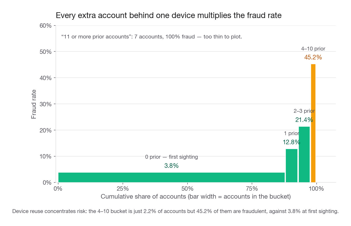
The as-of counter is strong on its own:
| Accounts already seen on this device | Accounts | Fraud rate |
|---|---|---|
| 0 (first sighting) | 84,523 | 3.84% |
| 1 | 4,817 | 12.85% |
| 2 to 3 | 4,524 | 21.37% |
| 4 to 10 | 2,129 | 45.23% |
| 11 or more | 7 | 100.00% |
Money and channel. Fraudulent first payments average 148.14 USD against 60.48 for legitimate ones, and the medians (87.30 against 40.33) say the gap is not one outlier. Credit as a funding source carries a 13.7 percent fraud rate against 3.8 for a bank transfer, which fits the mechanism: a stolen card number is easier to get than stolen bank credentials. Paid social signups run at 10.05 percent against 3.22 for referrals.
Interview tip: For every engineered feature, write one clause saying what real-world behaviour it encodes. "Accounts per device" is a column, "one phone, forty identities" is an argument, and the second is what the reviewer remembers.
Step 4: The split, and why a random one lies to you
This is the decision that separates a submission surviving contact with production from one that does not. Two separate things inflate the number a careless build reports, and only one of them is about the split.
Problem one: future information inside a feature. The whole-file device count already reflects accounts that have not registered yet, so no production scorer can compute it. Be precise about what repairs that, because nothing about the split does: under a time split, swapping whole-file counters for as-of ones still moves PR-AUC from 0.636 to 0.573. That 0.063 is future information sitting inside a column, and it survives every split you could write.
You will hear a neighbouring story called entity bleed: a shuffle spreads a crew's forty accounts across both sides and the model memorises a device rather than a behaviour. That hazard is real when you hand the model an entity identifier or an entity-level target encoding. It is not what happens here, and checking beats asserting. In the stable first nine weeks a crew-grouped split cuts the share of test-window ring accounts whose device was already seen in training from about 65 percent to 4 percent and address overlap from 57 percent to zero, and PR-AUC does not move: over six paired splits the random one scores 0.003 lower, standard error 0.010. With only counts in the feature matrix, there is no identity left to memorise.
Problem two: regime drift. This one is entirely about the split, and here it carries essentially all of it. Fraud tooling changes. Here the crews retool in the final month, and the change is dramatic even though the overall rate barely moves, from 5.92 percent to 6.33 percent.
| Fraud signature | First nine weeks | Final four weeks |
|---|---|---|
| Web platform share | 50.7% | 15.6% |
| Android platform share | 29.7% | 56.7% |
| Paid social channel share | 47.9% | 28.8% |
| Credit funding share | 55.3% | 22.0% |
| Debit funding share | 30.7% | 56.8% |
| Cashing out within one hour | 46.8% | 26.3% |
A random split lets the model see the new signature during training. A time split forces it to extrapolate, which is the job. Run all four combinations: crossing the counting rule with the split is far more persuasive than asserting leakage exists.
from sklearn.ensemble import HistGradientBoostingClassifier
from sklearn.metrics import average_precision_score

CATS = ["funding_source", "signup_channel", "platform", "network_type", "country"]
for c in CATS:
    df[c] = df[c].astype("category")
BASE = ["log_latency", "log_amount", "pay_hour"] + CATS
y = df.is_fraud.to_numpy()

def evaluate(count_cols, split):
    X = df[BASE + count_cols]
    if split == "time":
        train = np.arange(len(df)) < int(len(df) * 0.72)
    else:
        train = np.random.default_rng(7).random(len(df)) < 0.72
    m = HistGradientBoostingClassifier(max_iter=250, learning_rate=0.07,
                                       categorical_features=CATS, random_state=0)
    m.fit(X[train], y[train])
    p = m.predict_proba(X[~train])[:, 1]
    return m, X, y[~train], ~train, p, average_precision_score(y[~train], p)
Reported on the same cost basis we build in Step 7, the four combinations look like this. Cost per payment is the residual loss the policy leaves behind, in USD, at each configuration's own best threshold on its own test set. Treat that as a comparison convention, not a shipping number: every row gets the most flattering cut available to it, the naive one included. Step 7 picks a cut you are allowed to quote.
| Counting rule | Split | PR-AUC | Best threshold | Precision | Recall | Cost per payment |
|---|---|---|---|---|---|---|
| Whole-file counts | Random | 0.704 | 0.10 | 0.602 | 0.667 | 2.29 |
| Whole-file counts | Time | 0.636 | 0.07 | 0.512 | 0.607 | 3.37 |
| As-of counts | Random | 0.669 | 0.11 | 0.570 | 0.632 | 2.55 |
| As-of counts | Time | 0.573 | 0.13 | 0.487 | 0.531 | 4.12 |
Read the corners. The naive setup claims residual loss of 2.29 per payment. The honest one delivers 4.12, so reality is 80 percent worse than the claim. The split contributes more of that gap than the counting rule, and the two interact: repairing either alone recovers only part of it. Across 26,880 payments, believing the top row costs about 49,000 USD of unbudgeted loss a month. Pick every threshold on a validation slice instead and the rows shift a little, the naive one to 2.33 or 2.45 and the honest one to 4.12 or 4.23 depending on the slice, so the gap lands between 68 and 82 percent. Ordering and conclusion do not budge.
That paragraph, with those two numbers, is the most valuable thing you can put in a fraud write-up. It shows you treat the estimate as a forecast about the future rather than a description of the file.
When is the label actually known
Two refinements a strong candidate raises unprompted.
The split is on signup order, but the label is realised at payment time. Here 2,801 training rows, 4.05 percent of the training window and 147 of them fraudulent, carry a payment_ts later than the first test-window signup, so those outcomes would not have existed at a genuine refit. Median spill is 1.8 days, worst 19.9. Cutting on label-availability date is the cleaner frame, and measuring beats inflating: dropping those rows moves PR-AUC from 0.573 to 0.567 and cost per payment from 4.12 to 4.03, and splitting on payment_ts gives 0.567 and 3.98. Care, not a third leak, and the headline 0.573 stands.
The second one is bigger, and the brief quietly hides it. You were handed a clean is_fraud on every payment in a thirteen-week window. No real payments book has that. Chargeback and issuer-reversal rights run 60 to 120 days depending on the rail, and laundering labels come out of investigations that close later still, so the newest weeks are always partly labelled. The direction of the damage is the sharp part of the answer: the test window here is the final 26 days, the least matured slice, and an immature label records true fraud as legitimate, turning a correct high score into an apparent false positive. Measured precision and PR-AUC fall, and the cost sweep is pushed toward a threshold that is too high. Two standard remedies: hold the newest weeks back until the chargeback window closes and report the headline metric on a matured window, or keep them and treat the label as right-censored, reweighting by an observed maturation curve. Say which you would use.
Interview tip: When a reviewer asks "how do you know your model will hold up", the winning answer is a number that quantifies the gap between the optimistic setup and the honest one, not a sentence about how you were careful.
Step 5: Class imbalance, and the case for doing very little
Six percent positives triggers a reflex: resample, set class weights, reach for SMOTE. Resist long enough to ask what the imbalance actually breaks.
At 6 percent, a gradient boosted tree fits perfectly well. What breaks is anything depending on the 0.5 cutoff, because the model correctly learns that most first payments are fine and only 3.7 percent of the test book scores above 0.45. Evaluate with accuracy and you get 94 percent by predicting "clean" for everything, which is why accuracy is banned from this page.
Here is what each remedy actually does.
The sentence to write, and to say aloud: resampling changes the score scale, not the ranking, and since the operating point comes from a cost matrix anyway, the threshold sweep already does everything resampling would have done without breaking calibration.
If a follow-up pushes, be specific about SMOTE. It interpolates between neighbouring positives. Two positives here may be a card-testing crew on hosting infrastructure and a lone mule with a stolen debit card, and their midpoint is a payment nobody ever sent. On images that is defensible. On mixed categorical and count features it manufactures nonsense, and then you evaluate on it.
Step 6: Fit, and check the score before you trust it
The honest configuration, as-of counters and a time split, is the one we take forward.
FEATS = ["log_latency", "log_amount", "pay_hour",
         "prior_device_accounts", "prior_ip_accounts"] + CATS
X = df[FEATS]
train = np.arange(len(df)) < int(len(df) * 0.72)
model = HistGradientBoostingClassifier(max_iter=250, learning_rate=0.07,
                                       categorical_features=CATS, random_state=0)
model.fit(X[train], y[train])
p = model.predict_proba(X[~train])[:, 1]
te = df[~train].reset_index(drop=True)
yt, amt = y[~train], te.amount_usd.to_numpy()
print(len(te), round(yt.mean(), 4), round(average_precision_score(yt, p), 4))
26880 0.0634 0.5726Test window: 26,880 payments, 6.34 percent fraudulent. ROC AUC is 0.818, PR-AUC is 0.573. Quote the second with its floor beside it: random ranking scores a PR-AUC equal to the base rate, 0.063, so the model concentrates fraud at the top of the list about nine times better than chance. ROC AUC on a 6 percent problem flatters everything, which is why fraud teams do not lead with it.
Before touching thresholds, check whether the scores mean what they say. Bucket the test set into score deciles and compare the average prediction to the observed rate.
| Score decile | Mean predicted | Observed rate | Payments |
|---|---|---|---|
| 1 (lowest) | 0.0117 | 0.0152 | 2,690 |
| 5 | 0.0197 | 0.0242 | 2,688 |
| 7 | 0.0225 | 0.0416 | 2,690 |
| 8 | 0.0278 | 0.0436 | 2,686 |
| 9 | 0.0463 | 0.0577 | 2,688 |
| 10 (highest) | 0.4304 | 0.3650 | 2,688 |
Two honest problems, and naming them beats hiding them. In the middle deciles the model under-predicts, calling 2.3 percent where the truth is 4.2. In the top decile it over-predicts, calling 43 against a true 36.5. Both are the fingerprint of a model trained before a tooling change and tested after it: the old signature is over-weighted, and part of the new fraud drifted into the middle of the distribution.
The remedy belongs in the recommendations: refit weekly on a trailing window and recalibrate with isotonic regression on the most recent complete week. Be precise about what that buys, because this is where candidates over-claim. The fixed-threshold sweep in the next section does not need it: it minimises realised cost on labelled holdout payments, so it depends only on the order of the scores, and any strictly monotone recalibration relabels the winning cut while blocking the same payments for the same money. What does need a calibrated p is the amount-aware rule that follows the sweep, which reads the score as a per-payment probability.
Step 7: Turn the score into a decision with an explicit cost
This is what the prompt was really asking about. Write the cost matrix down before you touch a threshold, and state where each number came from, because the follow-up is always "where did that come from".
| Outcome | What happens at Tandem Pay | Cost |
|---|---|---|
| True negative | Payment goes through, everyone is happy | 0 |
| False negative | Fraud settles, funds leave, the issuer reverses, ops handles the dispute | amount plus 14 USD |
| False positive | A real user is blocked: support contact plus the share who never return | 22 USD |
| True positive | Fraud stopped before settlement | 0 |
The 14 USD is a dispute and operations fee. The 22 USD is what candidates hand-wave, so ground it: about 6 USD of support contact plus an expected 16 USD of lost contribution from blocked users who never come back. Whether those are exactly right matters far less than that you wrote them down and can re-run the sweep with the risk team's real ones.
Notice the asymmetry. A miss costs the amount, variable, averaging 148 USD on fraudulent payments. A false alarm costs a flat 22. Misses are roughly seven to eight times more expensive, so 0.5 is going to be badly wrong.
FN_FIXED, FP_COST = 14.0, 22.0
def total_cost(blocked):
    missed = (amt + FN_FIXED) * ((yt == 1) & ~blocked)
    upset = FP_COST * ((yt == 0) & blocked)
    return missed.sum() + upset.sum()

grid = np.round(np.arange(0.02, 0.96, 0.01), 2)
costs = np.array([total_cost(p >= t) for t in grid])
best = grid[costs.argmin()]
print(round(total_cost(np.zeros(len(yt), bool)), 0), best, round(costs.min(), 0))
277716.0 0.13 110740.0Blocking nothing costs 277,716 USD across the test window, or 10.33 per payment. The best threshold on this test set, 0.13, brings that to 110,740, a 60.1 percent reduction. Blocking everything costs 553,894, a useful anchor: a policy that fires too often is twice as expensive as no policy at all.
| Threshold | Payments blocked | Precision | Recall | Fraud USD stopped | Total cost |
|---|---|---|---|---|---|
| 0.05 | 3,552 | 0.294 | 0.613 | 78.4% | 119,116 |
| 0.10 | 2,164 | 0.429 | 0.545 | 70.7% | 112,349 |
| 0.13 | 1,857 | 0.487 | 0.531 | 69.0% | 110,740 |
| 0.20 | 1,470 | 0.581 | 0.501 | 65.3% | 113,550 |
| 0.30 | 1,215 | 0.663 | 0.473 | 61.5% | 119,230 |
| 0.50 | 944 | 0.786 | 0.436 | 55.9% | 129,890 |
| 0.70 | 782 | 0.887 | 0.408 | 52.9% | 135,757 |
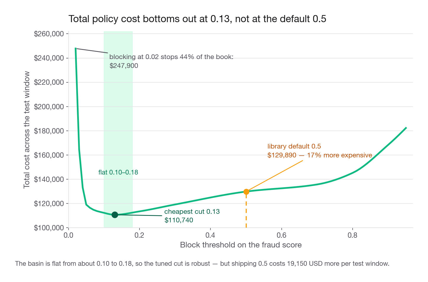
The library default of 0.5 costs 129,890 against 110,740, so it is 17 percent more expensive than the tuned cut. The curve is flat between roughly 0.10 and 0.18, itself worth a sentence: the threshold is not delicate, so a risk manager can move within that band to hit a capacity target without paying much.
Note the fifth column too. At 0.13 recall counted in payments is 53.1 percent, but recall counted in dollars is 69.0 percent, because the model ranks large fraud higher. Fraud teams are paid in dollars, so lead with the dollar figure and give the count beside it.
Do not read the winning cut off the test set
Look again at what that sweep did. The 0.13 was chosen by minimising cost on the same 26,880 payments the 110,740 is reported on, so the operating point is both selected and scored on the holdout. On a page arguing that you must evaluate on data resembling the future, that is the last leak standing. Pick the cut on a validation slice instead: fit on everything up to a fortnight before the training cutoff, sweep the cost curve on that fortnight, and only then look at test.
sig = df.signup_ts.to_numpy()
val = train & (sig >= sig[train][-1] - 14 * 86400)
sel = HistGradientBoostingClassifier(max_iter=250, learning_rate=0.07,
                                     categorical_features=CATS, random_state=0)
sel.fit(X[train & ~val], y[train & ~val])
pv, yv, av = sel.predict_proba(X[val])[:, 1], y[val], df.amount_usd.to_numpy()[val]
vcost = [((av + FN_FIXED) * ((yv == 1) & (pv < t))).sum()
         + FP_COST * ((yv == 0) & (pv >= t)).sum() for t in grid]
t_val = grid[int(np.argmin(vcost))]
print(int(val.sum()), t_val, round(total_cost(p >= t_val), 0))
14824 0.18 112387.0The fortnight picks 0.18, which costs 112,387 on test against the 110,740 the test-optimal cut achieves: 1.5 percent of optimism, or 4.18 per payment rather than 4.12. Vary the slice from one week to five and the pick wanders between 0.12 and 0.23 and the test cost between 110,740 and 113,812, so the penalty runs from nothing to 2.8 percent, median 1.5. It is that small for the reason you just noticed: on a flat cost surface, choosing the cut badly costs almost nothing. Quote 4.18 and say in one clause how you picked it.
Interview tip: A number you tuned on a dataset is not a result on that dataset. Sweep on a validation slice, report on test, and say plainly which is which.
The threshold should not be a single number
First settle the claim candidates get backwards, because the next rule is where it actually bites. Recalibration is not a prerequisite for thresholding.
mono = np.sqrt(p)                                    # any strictly increasing relabelling
print(bool(((mono >= np.sqrt(0.13)) == (p >= 0.13)).all()),
      round(total_cost(mono >= np.sqrt(0.13)), 0))
True 110740.0Same blocked set, same money, because the sweep reads the score only through its order. Isotonic regression relabels the winning cut from 0.13 to about 0.11 and lands at 110,632, a tenth of a percent away, and being only weakly monotone it pools ties and can coarsen the cuts available to you rather than improve them.
Now the rule that does depend on calibration. The cost of a miss scales with the amount, so a fixed cut is provably suboptimal. Block when expected loss beats expected annoyance, per payment: block if p * (amount + 14) > (1 - p) * 22.
odds = p / np.clip(1 - p, 1e-9, None)
amount_aware = odds > (FP_COST / (amt + FN_FIXED))
print(int(amount_aware.sum()), round(total_cost(amount_aware), 0))
1682 93876.0Fewer payments blocked and 15.2 percent less cost than the best possible fixed threshold. In score terms, a 900 USD transfer is stopped at roughly 0.024 while a 12 USD transfer runs until about 0.46. One line of arithmetic, and it beats every fixed cut. It also has no tuned parameter, worth saying out loud after the previous subsection: nothing was picked on the holdout, so 93,876 carries no selection penalty at all. The best simple policy here is the one that needed no tuning.
It is, however, the rule miscalibration breaks, and Step 6's two errors bite at opposite ends of it. Its implied cut is low for large payments and high for small ones, so the middle-decile under-prediction sits at the large-payment cut and the top-decile over-prediction sits at the small-payment cut. The raw rule therefore lets large risky payments through and blocks small ones it should not. Fit isotonic regression on the first half of the holdout and the blocks move exactly that way: the top amount decile goes from 801 blocked to 839, below-median amounts from 174 to 124, and cost from 93,876 to 89,138, a further 5.0 percent. Score only the untouched second half and the gain holds at 4.4 percent, so it is not an artefact of calibrating on the same rows.
Step 8: What the model is keying on, in a manager's language
The prompt asks you to explain the model to someone who neither wants nor needs the mathematics. Permutation importance on the test set, scored by PR-AUC, gives the honest answer: how much worse the ranking gets when each column is shuffled.
from sklearn.inspection import permutation_importance
r = permutation_importance(model, X[~train], yt, scoring="average_precision",
                           n_repeats=5, random_state=1, n_jobs=-1)
print(pd.Series(r.importances_mean, index=FEATS).sort_values(ascending=False).round(4))| Feature | Drop in PR-AUC when shuffled |
|---|---|
prior_ip_accounts | 0.395 |
prior_device_accounts | 0.070 |
log_amount | 0.052 |
log_latency | 0.021 |
signup_channel | 0.012 |
funding_source | 0.009 |
platform | 0.006 |
network_type | 0.002 |
country | 0.000 |
One feature carries most of the model. Shuffling the address reuse counter costs 0.395 of PR-AUC, five times the next feature and most of the entire lift over the 0.063 base rate.
Now the country row, the most interesting line in the table. Marginally, Germany looked three times riskier than Brazil. Conditionally, once the model knows how many accounts share the address, country contributes nothing. The country effect was never about countries: it was a shadow cast by hosting ranges that happen to be registered in a few places, and the reuse counter captures the underlying behaviour with far more precision.
That distinction is a policy decision as much as a modelling one. A country rule declines real users in Germany for something they did not do, is trivially defeated by a crew renting infrastructure elsewhere, and is hard to defend to a regulator. Say all three out loud. Fraud interviewers listen for whether you noticed.
The manager-facing paragraph, which goes nearly verbatim into the summary:
The model is not profiling people, it is profiling infrastructure and haste. It flags accounts sharing a phone or network address with accounts we have already seen, sending money within minutes of signing up rather than days, sending an unusually large first amount, and arriving through paid social on a funding instrument that is easy to steal. A user on their own phone and home network, sending 40 USD to a friend three days after installing, is essentially never flagged, and that is the overwhelming majority of our users.
Interview tip: When you find a feature that looks discriminatory but is really a proxy, say explicitly that you checked whether it survives conditioning and that you would not ship the rule. That single sentence separates you from every candidate who happily reported "country is predictive".
Step 9: The product answer, four score bands
Candidates rush this question and product managers read it first. "Block if the score is high" is not a product. Blocking is the most expensive action available and not the only one. Tandem Pay has four levers in ascending order of friction: let it through, let it through and watch, hold for a document or selfie check, and decline with a manual appeal path. Match each to a band. Round illustrative edges first, at 0.02, 0.13, and 0.45, and then optimise them:
| Band | Score | Payments | Share of book | Fraud rate | Share of fraud cases | Share of fraud USD |
|---|---|---|---|---|---|---|
| Clear | below 0.02 | 15,144 | 56.3% | 2.05% | 18.3% | 6.3% |
| Watch | 0.02 to 0.13 | 9,879 | 36.8% | 4.93% | 28.6% | 24.7% |
| Step up | 0.13 to 0.45 | 868 | 3.2% | 17.63% | 9.0% | 12.0% |
| Decline | above 0.45 | 989 | 3.7% | 76.04% | 44.2% | 57.0% |
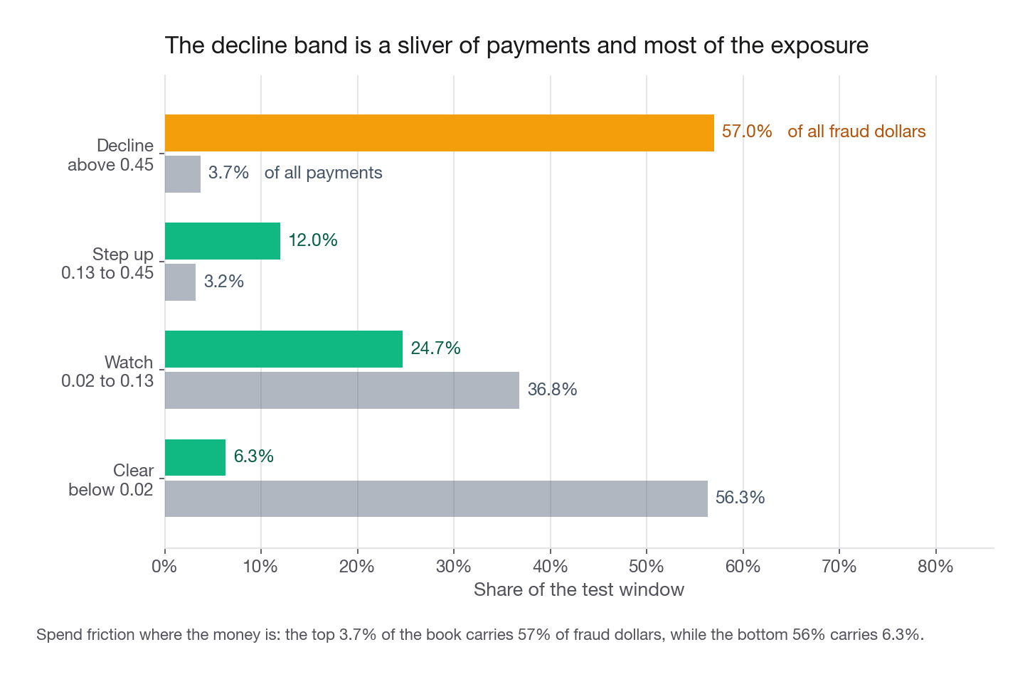
The last two columns are the argument. The top 3.7 percent of the book carries 57 percent of the fraud dollars at 76 percent precision, so declining there is easy to defend: three in four are genuinely fraud and the fourth gets an appeal. The bottom 56 percent carries 6.3 percent of the exposure, so friction placed there is almost pure cost.
Then make the step-up band pay for itself. A document check costs about 4 USD rather than 22 and stops roughly 72 percent of the fraud routed to it, because crews abandon rather than complete a verification. Write that cost down as code, because "who pays the 4 USD" is the next question a reviewer asks and the three defensible answers differ by more than a percent. The consistent one: everybody who completes a check pays for it, so every real user routed there plus the 28 percent of routed fraud that does not abandon.
CHECK, STOP = 4.0, 0.72          # document check; share of routed fraud that abandons
def ladder_cost(t1, t2):
    band, dec, allow = (p >= t1) & (p < t2), p >= t2, p < t1
    loss = amt + FN_FIXED
    return (loss[(yt == 1) & allow].sum()                    # fraud let through
            + CHECK * ((yt == 0) & band).sum()               # checks on real users
            + CHECK * (1 - STOP) * ((yt == 1) & band).sum()  # checks fraud completes
            + (1 - STOP) * loss[(yt == 1) & band].sum()      # fraud surviving a check
            + FP_COST * ((yt == 0) & dec).sum())             # real users declined

pairs = [(a, b) for a in grid for b in grid if b > a]
t1, t2 = min(pairs, key=lambda ab: ladder_cost(*ab))
print(t1, t2, round(ladder_cost(t1, t2), 0))
0.03 0.24 92252.0Jointly optimising the two cuts gives 0.03 and 0.24, totalling 92,252, or 16.7 percent better than the best single block threshold on the same test set. Both are read off the holdout, so treat 16.7 percent as a ceiling rather than a forecast. Repeat the selection on Step 7's validation fortnight and it returns 0.04 and 0.25, costing 94,407 on test: 3.51 per payment, 16.0 percent better than the honestly chosen single cut of 0.18.
Two independent refinements, amount-aware thresholds at 93,876 and a graded ladder at 92,252, land 1.73 percent apart. Not a coincidence: both spend friction in proportion to exposure instead of applying one blunt rule everywhere. The honest version carries a second lesson. The ladder fits two cuts and the amount-aware rule fits none, so once both are chosen the way production forces you to choose them, the ladder lands at 94,407 against the untuned rule's 93,876 and the ranking quietly flips. Every parameter you pick on a holdout charges rent.
That last bullet is the follow-up interviewers love. Decline everything above 0.45 and you never learn whether those payments were fraud, so the training data rots into a description of the fraud you allow rather than the fraud that exists. Releasing a small random slice, or scoring successful appeals, is the standard fix, and raising it unprompted signals you have run a model in production and not only in a notebook.
What goes in the write-up
Five sentences, at the top, before any chart.
A model on first payments reaches PR-AUC 0.573 on a forward-in-time holdout against a 0.063 base rate, and 0.573 is the number to plan with: the whole-file, randomly split version reports 0.704 and will not reproduce.
Blocking above a score of 0.18, chosen on a validation slice and only then measured on the holdout, cuts residual fraud cost by 60 percent, from 10.33 to 4.18 USD per payment.
Replacing the fixed cut with an amount-aware rule, or with a graded step-up band whose two cuts are chosen the same honest way, takes that to 3.49 and 3.51 USD per payment respectively, a further 16 percent.
The single strongest signal is reuse of a network address across accounts, followed by device reuse and payment amount, and country adds nothing once reuse is known, so no country rule should ship.
Ship in shadow mode for two weeks, refit weekly, and randomly release a sample of the decline band to keep labels alive.
Every one has a number and an action. Compare the version most candidates submit: "we built a random forest with 95 percent accuracy and identified several important features." Same model, entirely different verdict.
Common traps
Reporting accuracy. Predicting "clean" for every payment scores 94 percent here. If accuracy appears in your summary the reviewer stops reading. Use PR-AUC, precision and recall at your operating point, and cost.
Whole-file aggregate features. Any
transform("size"), mean, or count over the full frame smuggles the future into training. Sort by time and usecumcountor an expanding window. Under a time split this leak alone is worth 0.063 of PR-AUC and roughly 20,000 USD a month of hidden loss.Random splits on time-stamped fraud. The signature drifts, so a shuffle hands the model next month's fraud during training. Split on a date, and if the challenge forbids it, say in one line what you would have found.
Picking the operating point on the test set. Sweeping a threshold on the holdout and then reporting that holdout's cost is selection on the same rows. It costs 0 to 2.8 percent here, small only because the curve is flat, which you cannot know until you check. Pick the cut on a validation slice and say you did.
Treating the newest weeks as fully labelled. Chargebacks and investigations land 60 to 120 days late, so recent data under-reports fraud and measured precision looks worse than the truth. Report the headline metric on a matured window.
Accepting the 0.5 cutoff. It is a library default chosen so that
predictcan exist, not a business decision. With a seven-to-one cost asymmetry it is 17 percent more expensive than the right cut.Imputing away the unresolved country. Those 6.4 percent of addresses carry an 11.8 percent fraud rate. Keep the missingness as a level and name it.
Reaching for SMOTE at 6 percent positives. Interpolating between two unrelated fraud patterns manufactures payments nobody sent. Tune the threshold instead.
Shipping a country rule because country looked predictive. It was a proxy for hosting infrastructure and it dies the moment you condition on address reuse. Check for it and say you checked.
Ignoring the label feedback loop. Blocked payments produce no outcome, so an unmonitored decline band poisons the next training set.
Handing over a score with no action attached. The prompt asks what the app should do. Score bands mapped to concrete product behaviour is the answer, and that section is the one most likely to be read aloud in the debrief.
Quick self-check
Answer these out loud, in full sentences, before you call the project finished.
The four-cell table crosses the counting rule with the split. How much PR-AUC does each axis account for, and why does repairing the split alone still leave 0.063 on the table?
Your cost matrix charges the amount plus a fixed fee for a miss and a flat fee for a false alarm. Derive the block rule from expected value, and explain why it produces a different threshold for a 12 USD payment than for a 900 USD one.
The unresolved country bucket is 6.4 percent of accounts with roughly triple the base fraud rate. What are you claiming about the world when you keep it as its own level, and what would falsify that claim?
Address reuse dominates the importance table. What does a crew do next month to defeat it, and which feature still fires?
Your top score decile predicts 43 percent and observes 36.5 percent. Does that break the ranking, the threshold arithmetic, or both, and what is the fix?
Your labels come from chargebacks and investigations that close weeks after the payment. What fraction of your final month is fully matured, which direction does that bias the precision you report, and what would you report instead?
If question 2 or question 5 comes slowly, rebuild those two cells. They are where the onsite panel pushes hardest, because they are where a candidate either reasons in expected value or does not.