7.2 Cohorts, Power Users, Running Totals, and Ranking
Find the core decision, design, or behavior signal.
Turn the lesson into a concise response blueprint.
Name the trap you would avoid in a real interview.
Use these checkpoints as your reading path before diving into the full lesson.
- 1Why this matters in interviews
- 2The order log you are handed
- 3Pattern 5: the cohort grid
- 4The problem as stated
- 5The three definitions to pin down
The previous lesson measured the space between rows. This one measures accumulation: how a group of accounts that arrived together behaves over the following weeks, when somebody crosses a threshold worth caring about, how a number piles up day by day, how to guess a month's total from twelve days of it, and how to rank people inside their own group without the ranking function changing your answer.
Why this matters in interviews
Nobody asks for a cohort query because they want a cohort query. They ask because it forces you to declare four things you would rather leave vague: who is in the group, what the clock starts on, what counts as still being here, and which cells you may read. A candidate who writes the query and then reads every cell has failed the question with correct SQL.
The rest works the same way. "When did this account become a power user" is a threshold question and nobody told you what the threshold counts. "Running total by day" is a frame question and the standard's default frame is not the one you want. "Estimate the month" is seasonality wearing a division sign.
Weak version: "I grouped by signup month and counted active users per week, here is the table." Strong version: "I counted accounts with at least one order in each week since signup. Note first that the June cohort has between zero and twenty nine days of history, so every June cell past week zero is a partial numerator over a full denominator. I would read March through week twelve, April through week seven, May through week three, and leave June off the chart until July closes."
The second costs eleven extra seconds and is the whole interview.
Interview tip: Say which cells of a cohort table are readable before saying what the numbers mean. Refusing to interpret a censored cell scores higher than finding a clever story in it.
The order log you are handed
We stay with Kestrel, the fictional recipe app with a grocery cart bolted on, and move from its screen-view log to its two commercial tables.
Column in users | Type | What it holds |
|---|---|---|
user_id | int | Account key, joins to orders |
signup_date | date | Day the account was created, no time component |
country | text | One of US, CA, UK, IE, SG, NZ |
channel | text | organic, paid, or referral acquisition source |
Column in orders | Type | What it holds |
|---|---|---|
order_id | bigint | Monotonic key, unique across the table |
user_id | int | Account that placed the order |
ordered_at | timestamp | When checkout completed, to the second |
amount_usd | numeric | Basket total in dollars |
item_count | int | Line items in the basket |
Two derived exports also appear, orders_may and orders_jun, the May and June slices handed over as separate files, because finance exports one per accounting period and nobody reconciles them until a question spans both. This block builds everything deterministically from pandas and numpy, and every figure below comes out of it.
import numpy as np
import pandas as pd

SEED = 51197
rng = np.random.default_rng(SEED)
N_USERS, HORIZON, TAU = 9000, 122, 45.0
START = pd.Timestamp("2026-03-01")                       # day 0, a Sunday

signup_day = rng.integers(0, HORIZON, N_USERS)
users = pd.DataFrame({
    "user_id": np.arange(1, N_USERS + 1),
    "signup_date": START + pd.to_timedelta(signup_day, "D"),
    "country": rng.choice(["US", "CA", "UK", "IE", "SG", "NZ"], N_USERS,
                          p=[.52, .17, .14, .07, .06, .04]),
    "channel": rng.choice(["organic", "paid", "referral"], N_USERS, p=[.55, .31, .14]),
})

exposure = (HORIZON - signup_day).astype(float)          # days we can still observe them
rate = rng.gamma(2.0, 0.085, N_USERS)                    # orders per day just after signup
n_orders = rng.poisson(rate * TAU * (1.0 - np.exp(-exposure / TAU)))

buyer = np.repeat(users.user_id.values, n_orders)
base = np.repeat(signup_day, n_orders).astype(float)
u = rng.random(buyer.size)
day = base - TAU * np.log1p(-u * (1.0 - np.exp(-np.repeat(exposure, n_orders) / TAU)))
dow = (np.floor(day).astype(np.int64) + 6) % 7           # 0 = Monday ... 6 = Sunday
shifted = day + (5 + (rng.random(buyer.size) < 0.45) - dow)
shifted = np.where(shifted >= HORIZON, shifted - 7.0, shifted)
pull = (rng.random(buyer.size) < 0.22) & (dow < 5) & (shifted >= base)
day = np.where(pull, shifted, day)                       # weekend grocery habit

orders = pd.DataFrame({
    "user_id": buyer,
    "ordered_at": START + pd.to_timedelta((day * 86400).astype(np.int64), "s"),
    "amount_usd": np.round(rng.lognormal(3.5, 0.62, buyer.size), 2),
    "item_count": rng.poisson(4.2, buyer.size) + 1,
}).sort_values(["user_id", "ordered_at"], kind="stable").reset_index(drop=True)
orders.insert(0, "order_id", np.arange(1, len(orders) + 1))
orders_may = orders[orders.ordered_at.dt.month == 5].copy()
orders_jun = orders[orders.ordered_at.dt.month == 6].copy()
That gives 45,185 orders from 9,000 accounts across 122 consecutive days, 1 March through 30 June 2026, worth 1,809,944 dollars. Of those accounts 7,840 ordered at least once and 1,160 never did. The May export holds 14,444 rows, June 15,168.
Three properties matter later. Order rate decays after signup, so a fresh account is busiest in its first fortnight. About a fifth of weekday orders get dragged onto the following weekend, making Saturday and Sunday worth roughly double a weekday. And the window ends hard on 30 June, so an account created on 25 June has five days of history while one created on 2 March has a hundred and twenty. That last one is the villain of the next two patterns. Register these frames in DuckDB or SQLite under the names above to run the SQL yourself.
Pattern 5: the cohort grid
The problem as stated
"Group accounts by signup month and show what share of each placed an order in their first week, second week, and so on. Is retention getting better or worse?"
The three definitions to pin down
The grouping is who belongs together: signup month by default, though a cohort defined by first purchase silently drops everyone who never purchased, and interviewers probe that. The clock is what week zero means: calendar weeks compare cohorts on the same date and suit a mix-shift question, while weeks since signup compare them at the same age, which is what "their first week" asks for. The activity rule is what counts as present: one order is usual, and one order above some value or a single session each give a different curve.
The query
WITH activity AS (
  SELECT u.user_id,
         DATE_TRUNC('month', u.signup_date) AS cohort,
         CAST(FLOOR(DATE_DIFF('day', u.signup_date,
                              CAST(o.ordered_at AS DATE)) / 7.0) AS INT) AS week_no
  FROM users u
  JOIN orders o USING (user_id)
),
sizes AS (
  SELECT DATE_TRUNC('month', signup_date) AS cohort, COUNT(*) AS cohort_size
  FROM users GROUP BY 1
)
SELECT a.cohort, a.week_no, s.cohort_size,
       COUNT(DISTINCT a.user_id) AS buyers,
       ROUND(100.0 * COUNT(DISTINCT a.user_id) / s.cohort_size, 1) AS pct
FROM activity a JOIN sizes s USING (cohort)
WHERE a.week_no BETWEEN 0 AND 5
GROUP BY 1, 2, 3
ORDER BY 1, 2;
Two details carry weight. The denominator comes from users, not orders, so accounts that never bought stay in it. And the bucket is FLOOR(days / 7.0), not CAST(days / 7 AS INT): several engines round a double-to-integer cast rather than truncating, so day four lands in week one and week zero silently shrinks to four days wide. I wrote it the wrong way preparing this lesson; week zero came out lower than week one, and that impossibility was the only reason I caught it.
| Cohort | Size | Wk 0 | Wk 1 | Wk 2 | Wk 3 | Wk 4 | Wk 5 |
|---|---|---|---|---|---|---|---|
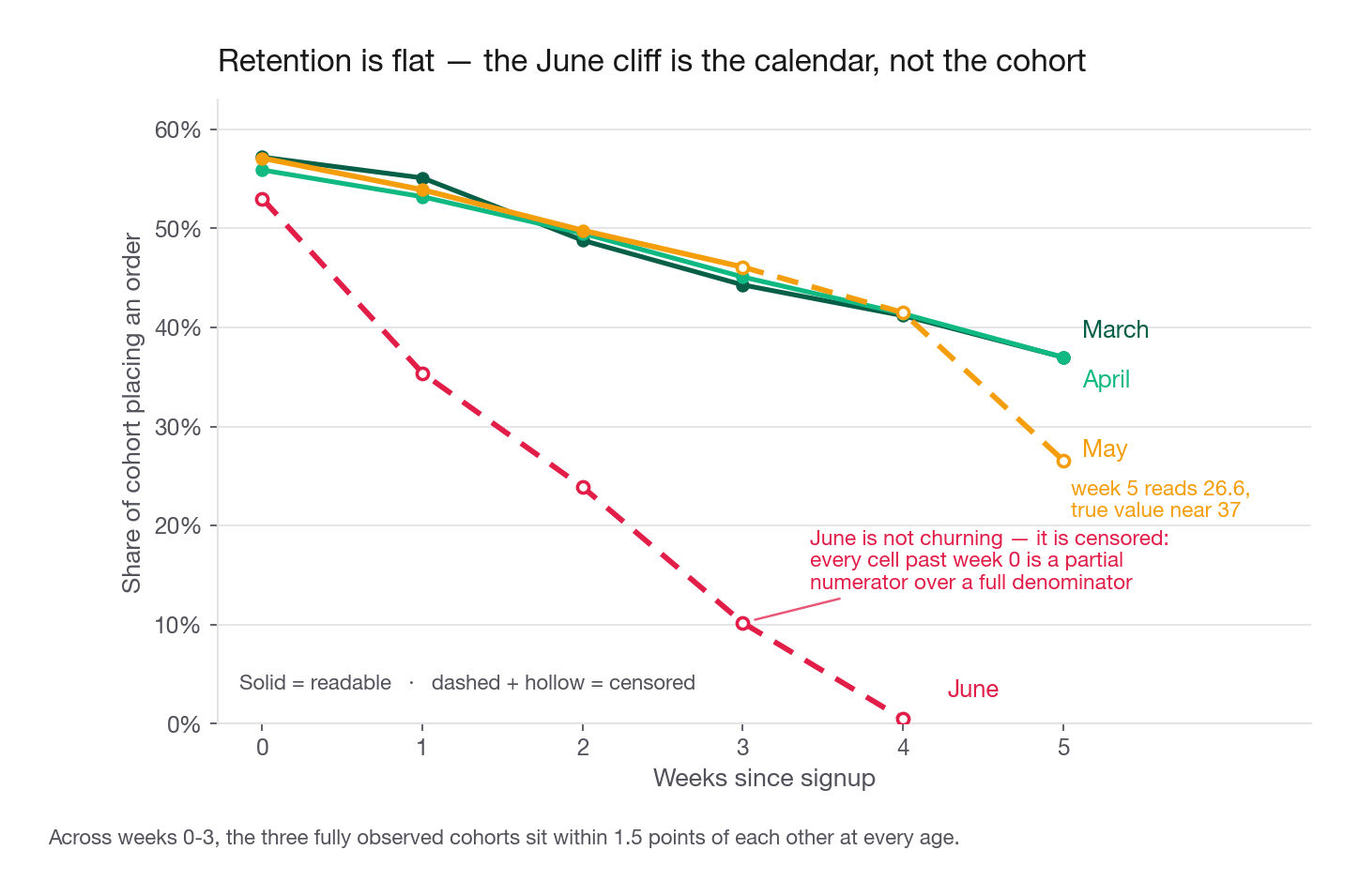
| March | 2,312 | 57.2 | 55.1 | 48.8 | 44.3 | 41.2 | 37.0 |
| April | 2,223 | 55.9 | 53.2 | 49.5 | 45.1 | 41.4 | 37.0 |
| May | 2,235 | 57.1 | 53.9 | 49.8 | 46.1 | 41.5 | 26.6 |
| June | 2,230 | 53.0 | 35.4 | 23.9 | 10.2 | 0.5 |
Reading it without embarrassing yourself
Look at June. It falls off a cliff, and a careless candidate calls the cohort terrible. It is not. Every June account has at most twenty nine days of history and some have zero, so June's week one counts only accounts created before 24 June, while its denominator is all 2,230.
The fix is mechanical: take each cohort's MIN(DATE_DIFF('day', signup_date, DATE '2026-06-30')), floor-divide by seven, and read only the weeks that fit inside it.
| Cohort | Min days observed | Complete weeks | Readable weeks |
|---|---|---|---|
| March | 91 | 13 | 0 through 12 |
| April | 61 | 8 | 0 through 7 |
| May | 30 | 4 | 0 through 3 |
| June | 0 | 0 | none |
Now the table means something. Across weeks zero to three the three readable cohorts sit within a point and a half of each other at every age. Retention is flat, and the apparent collapse was the calendar.
Notice that May's week four, 41.5, looks healthy beside March's 41.2 even though the rule says it is already contaminated. Contamination grows rather than announcing itself: week four is missing two days for the latest signups only, so it is nearly right, while week five is missing nine days for most of the cohort and reads 26.6 against a true value near 37. Trust your eye and you catch week five and ship week four.
Pattern 6: the day someone became a power user
The problem as stated
"We call an account a power user once it has bought ten times. For every account that got there, give me the date it happened."
This is a nomination, not a filter: pick one ranked row per account and report its timestamp.
SELECT user_id, ordered_at AS became_power_user
FROM (
  SELECT user_id, ordered_at,
         ROW_NUMBER() OVER (PARTITION BY user_id
                            ORDER BY ordered_at, order_id) AS nth_order
  FROM orders
) ranked
WHERE nth_order = 10
ORDER BY user_id;
Everything hangs on the ten in the WHERE. Rank each account's orders oldest first, keep the tenth. Accounts that never got there produce no row, which is what the prompt wants. The order_id tie-break matters because two baskets can share a second, and without it "the tenth order" is whichever row the engine emitted first.
| user_id | became_power_user |
|---|---|
| 3 | 2026-04-25 19:42:37 |
| 7 | 2026-06-26 09:16:37 |
| 8 | 2026-04-23 14:43:36 |
1,371 accounts qualify, 15.2 percent of the base. Median time from signup to promotion is 39 days, mean 42.8, fastest seven.
The definition question to raise unprompted
"Bought ten times" is ambiguous and the interviewer knows it. Ten orders, or ten items? Kestrel baskets average just over five items, so the readings are not close.
Both counters live in one CTE. Keep the ROW_NUMBER above and add a cumulative sum beside it, SUM(item_count) OVER (PARTITION BY user_id ORDER BY ordered_at, order_id ROWS UNBOUNDED PRECEDING) AS items_to_date, then count distinct users where each counter crosses ten.
Ten orders gives 1,371 accounts. Ten cumulative items gives 6,261, four and a half times as many, 70 percent of the base. A badge 70 percent of accounts hold is not a badge. Propose orders: a repeat purchase is a habit, a big basket is one decision.
The follow-up that catches people
"Is the power user rate improving? Break it out by cohort."
The obvious query counts, per cohort, how many accounts ever reached ten. Beside it, the same thing inside a fixed thirty day window from each account's own signup date.
| Cohort | Accounts | Min days observed | Percent ever promoted | Percent promoted within 30 days |
|---|---|---|---|---|
| March | 2,312 | 91 | 26.4 | 6.1 |
| April | 2,223 | 61 | 19.7 | 5.5 |
| May | 2,235 | 30 | 12.9 | 6.8 |
| June | 2,230 | 0 | 1.6 | 1.6 |
The naive column says power user creation collapsed from 26 percent to under 2 percent in four months, a five alarm fire. The windowed column says it has been flat near six percent throughout. The naive column is measuring how long we have been watching: March had ninety more days to accumulate a tenth order.
June reads 1.6 in both, because a thirty day window is not observable for anyone who joined in June. If the business needs a read before July closes, shorten it: five orders within fourteen days is observable for the 1,200 June accounts created on or before 16 June, and lands at 11.8 percent against 13.1, 11.0 and 12.0 for the earlier cohorts. That is the general move, wait or redefine to fit the time you have.
Worth volunteering too: those 1,371 power users generated 757,609 dollars of the 1,809,944 total, 41.9 percent of revenue from 15.2 percent of accounts.
Interview tip: Any rate shaped like "share of users who ever did X" is a cross-cohort trap. Rewrite it as "share who did X within N days of signup", N being the largest the youngest cohort supports.
Pattern 7: running totals and the frame you did not specify
The problem as stated
"Here are two files, May orders and June orders. Give me total spend per account across both, then spend to date for every day an account transacted."
Part one, and the union that eats rows
Stack the two exports in a CTE, then GROUP BY user_id with COUNT(*) and SUM(amount_usd). The only decision that matters is the stacking operator: UNION ALL, never bare UNION. UNION deduplicates whole projected rows, which here is silent data loss, because one account can genuinely place two baskets at the same value, as fourteen accounts here did. Get the mechanism right out loud: two different accounts at the same value are safe, their user_id differs, and 5,759 amounts here are shared across accounts without one being deduplicated.
Comparing whole rows means the counts depend on the projection, here the (user_id, amount_usd) pair GROUP BY needs: 29,612 rows with ALL and 29,598 without, so plain UNION deletes fourteen real orders. Carry order_id through and every row is unique again and the trap disappears. Nor is it the files overlapping: eight of the fourteen sit inside one export. Fourteen in thirty thousand never shows up in a spot check, which is why it is dangerous.
Part two, the cumulative version
The instinct is a windowed SUM on raw order rows. Resist it: "for every day" means an account with two baskets on one date should produce one row.
WITH daily AS (
  SELECT user_id, CAST(ordered_at AS DATE) AS order_date,
         COUNT(*) AS orders, SUM(amount_usd) AS day_spend
  FROM orders
  GROUP BY 1, 2
)
SELECT user_id, order_date, orders,
       ROUND(day_spend, 2) AS day_spend,
       ROUND(SUM(day_spend) OVER (PARTITION BY user_id
                                  ORDER BY order_date
                                  ROWS BETWEEN UNBOUNDED PRECEDING
                                           AND CURRENT ROW), 2) AS spend_to_date
FROM daily
ORDER BY user_id, order_date;
Aggregate to the grain the question asks for, then accumulate over it. Account 20 placed eight baskets, two on 13 June, and that pair collapses into one row:
| order_date | orders | day_spend | spend_to_date |
|---|---|---|---|
| 2026-06-11 | 1 | 55.16 | 55.16 |
| 2026-06-13 | 2 | 86.46 | 141.62 |
| 2026-06-15 | 1 | 17.16 | 158.78 |
| 2026-06-17 | 1 | 15.07 | 173.85 |
| 2026-06-19 | 1 | 18.97 | 192.82 |
| 2026-06-21 | 1 | 15.27 | 208.09 |
| 2026-06-26 | 1 | 29.79 | 237.88 |
Two checks catch a table with a row missing: spend_to_date must equal the row above plus this row's day_spend, 55.16 plus 86.46 giving 141.62 on to 237.88, and row count must equal distinct order dates, seven against eight raw orders.
ROWS versus RANGE, demonstrated
Skip the pre-aggregation and the frame becomes visible. Account 33's baskets include two same-day pairs; here is the running total both ways over raw rows ordered by date:
| order_date | amount_usd | ROWS frame | RANGE frame |
|---|---|---|---|
| 2026-06-06 | 42.52 | 42.52 | 73.65 |
| 2026-06-06 | 31.13 | 73.65 | 73.65 |
| 2026-06-17 | 63.24 | 136.89 | 167.02 |
| 2026-06-17 | 30.13 | 167.02 | 167.02 |
| 2026-06-19 | 40.17 | 207.19 | 207.19 |
RANGE treats every row sharing an ORDER BY value as a peer group and gives them all the same total, so the first 6 June row already shows 73.65, the sum of both, while ROWS counts physical rows and shows 42.52. Neither is wrong; they answer different questions. The trap is that an ordered window with no frame clause defaults to RANGE, so you get peer behaviour without asking for it.
| Frame clause | What accumulates | When you want it |
|---|---|---|
ROWS BETWEEN UNBOUNDED PRECEDING AND CURRENT ROW | Every physical row up to this one | Running totals, each row its own event |
RANGE BETWEEN UNBOUNDED PRECEDING AND CURRENT ROW | Every row whose sort key is at or before this one | Day-level totals when duplicates share a date |
ROWS BETWEEN 6 PRECEDING AND CURRENT ROW | This row and the six rows before it | Trailing seven day averages on a dense series |
Two failure modes live nearby. Drop PARTITION BY user_id and the frame stops caring whose row it is: it accumulates every daily row preceding this one in the window's ORDER BY. Order that unpartitioned window by user_id, order_date and account 39's first day opens at 9,850.40 instead of 74.74, having inherited every account ahead of it in the sort, not just the one above it. Leave the ordering as ORDER BY order_date alone and it is worse and unreproducible too: 367 daily rows share 12 May 2026, ROWS breaks those ties however the engine emits them, and repeated runs of the same query gave me values between 833,000 and 839,000, indefensible if asked. And a trailing window counts rows, not days, so on a sparse calendar 6 PRECEDING can span three weeks.
Where you filter changes what the window sees
WITH daily AS (
  SELECT CAST(ordered_at AS DATE) AS order_date, SUM(amount_usd) AS revenue
  FROM orders GROUP BY 1
),
rolled AS (
  SELECT order_date, revenue,
         AVG(revenue) OVER (ORDER BY order_date
                            ROWS BETWEEN 6 PRECEDING AND CURRENT ROW) AS trailing_7d,
         SUM(revenue) OVER (ORDER BY order_date
                            ROWS UNBOUNDED PRECEDING) AS revenue_to_date
  FROM daily
)
SELECT * FROM rolled
WHERE order_date BETWEEN DATE '2026-06-08' AND DATE '2026-06-14'
ORDER BY order_date;
The filter sits in the outer select on purpose. Move that WHERE into the daily CTE and the window sees only seven rows, so 8 June reports a trailing average of 13,549, its own value with nothing before it, rather than the correct 19,745, and revenue to date reads 13,549 instead of 1,360,959. Both look plausible; the second is wrong by two orders of magnitude.
| order_date | revenue | trailing_7d | revenue_to_date |
|---|---|---|---|
| 2026-06-08 | 13,549 | 19,745 | 1,360,959 |
| 2026-06-14 | 29,192 | 20,035 | 1,487,655 |
Interview tip: Write the frame clause every single time, even when the default is right. It costs six words and is the clearest signal that you know windows have frames at all.
Pattern 8: estimating a month from a partial month
The problem as stated
"It is the evening of Friday 12 June. The VP wants a June revenue number for Monday's board deck. Give her one and tell her how wrong it might be."
The query takes four lines; the reasoning takes the rest of the answer.
SELECT ROUND(SUM(amount_usd), 0) AS revenue_to_date,
       COUNT(DISTINCT CAST(ordered_at AS DATE)) AS days_elapsed,
       ROUND(SUM(amount_usd) / COUNT(DISTINCT CAST(ordered_at AS DATE)) * 30, 0)
         AS naive_full_month
FROM orders
WHERE ordered_at >= DATE '2026-06-01' AND ordered_at < DATE '2026-06-13';
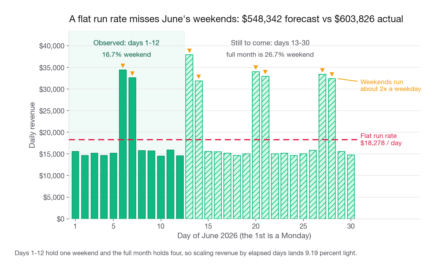
June 1 through 12 brought 219,337 dollars over twelve days. Scale by thirty over twelve and you forecast 548,342. June closed at 603,826. You are light by 55,484 dollars, 9.19 percent, and you would have told the board revenue fell month over month when it rose.
The reason is the calendar. June 2026 opens on a Monday, so days one through twelve hold exactly one Saturday and one Sunday, 16.7 percent weekend, while the full month holds four of each, 26.7 percent. And Kestrel is a grocery product.
In May every weekday averaged between 13,843 and 14,260 dollars, about three quarters of the month's 18,596 dollar daily average, while Saturday averaged 29,099 and Sunday 27,040, indices of 1.57 and 1.45. Weekends are worth 1.99 times a weekday, and your twelve day sample is short on exactly the days that carry the revenue.
The fix: reweight by the calendar, not the day count
Learn a weekday shape from a prior period, then ask what fraction of a full June it puts in the days you have seen.
WITH may_shape AS (
  SELECT DAYOFWEEK(CAST(ordered_at AS DATE)) AS dow,
         SUM(amount_usd) / COUNT(DISTINCT CAST(ordered_at AS DATE)) AS dow_mean
  FROM orders
  WHERE ordered_at >= DATE '2026-05-01' AND ordered_at < DATE '2026-06-01'
  GROUP BY 1
),
june AS (
  SELECT d::DATE AS cal_date, DAYOFWEEK(d::DATE) AS dow
  FROM GENERATE_SERIES(DATE '2026-06-01', DATE '2026-06-30', INTERVAL 1 DAY) AS t(d)
)
SELECT ROUND(219337.0 * SUM(dow_mean)
             / SUM(CASE WHEN cal_date < DATE '2026-06-13' THEN dow_mean ELSE 0 END), 0)
       AS weekday_adjusted_forecast
FROM june JOIN may_shape USING (dow);
That returns 595,241, an error of 1.42 percent instead of 9.19. May's weekday shape assigns 36.85 percent of a June to its first twelve days; a flat run rate assumes 40.
| Method | June forecast | Error | What it assumes |
|---|---|---|---|
| Run rate, PTD over 12 times 30 | 548,342 | -9.19 percent | Every day is worth the same |
| Prior month's share of its first 12 days | 596,060 | -1.29 percent | June's shape resembles May's |
| Weekday mix reweight from May | 595,241 | -1.42 percent | Weekday effect stable, level may drift |
| Trailing 7 days times a weekday index | 601,014 | -0.47 percent | Recent level, stable weekday effect |
The last wins because it does the two jobs separately: level from June's most recent full week, which already reflects growth, and shape from May, which has enough history to estimate a weekday index cleanly. The other three conflate the two.
The point the interviewer is actually testing
The naive run rate is not biased. It is unstable, which is worse, because it is right often enough to feel safe.
| Cut point | Day of week | Naive error | Weekday-adjusted error |
|---|---|---|---|
| After 7 days | Sunday | +0.28 percent | -1.17 percent |
| After 10 days | Wednesday | -7.41 percent | -2.33 percent |
| After 12 days | Friday | -9.19 percent | -1.42 percent |
| After 21 days | Sunday | -0.17 percent | -1.62 percent |
Cut on a Sunday and the naive method is nearly perfect, because a whole number of weeks holds the right weekday mix by construction. Cut on a Wednesday and it is off by seven percent, while the adjusted method stays inside two and a half percent everywhere. A method whose error depends on which weekday somebody asked you is not a method.
Interview tip: Whenever you divide by elapsed days and multiply by period length, name which days are missing from the numerator. That turns a wrong answer into a method with a stated assumption.
Pattern 9: the median you write yourself
The problem as stated
"Take only orders placed on the same calendar day the account signed up. Report the average and median basket. Do not use a percentile function."
The join condition is the fiddly part. ordered_at is a timestamp and signup_date is a date, so cast one side down; compare them directly and you match only orders placed at exactly midnight.
The trick: two row numbers that meet in the middle
Number rows ascending by amount, number them descending, keep rows whose two numbers are within one of each other. On an odd count exactly one row survives, the true middle. On an even count exactly two survive, and averaging them is the standard definition.
| Values | n | Ascending pos | Descending pos | Kept |
|---|---|---|---|---|
| 10, 20, 30, 40, 50 | 5 | 3 | 3 | the 30 alone |
| 10, 20, 30, 40 | 4 | 2 and 3 | 3 and 2 | 20 and 30, averaged to 25 |
Rather than a second sort, derive the descending number: a row at ascending position k of n sits at n - k + 1 from the other end, and one COUNT(*) OVER () gives n.
WITH first_day AS (
  SELECT o.amount_usd
  FROM orders o
  JOIN users u ON o.user_id = u.user_id
  WHERE CAST(o.ordered_at AS DATE) = u.signup_date
),
positioned AS (
  SELECT amount_usd,
         ROW_NUMBER() OVER (ORDER BY amount_usd) AS pos_asc,
         COUNT(*) OVER () AS n,
         COUNT(*) OVER () - ROW_NUMBER() OVER (ORDER BY amount_usd) + 1 AS pos_desc
  FROM first_day
)
SELECT MAX(n) AS first_day_orders,
       ROUND(AVG(amount_usd), 2) AS mean_usd,
       ROUND(AVG(CASE WHEN ABS(pos_asc - pos_desc) <= 1
                      THEN amount_usd END), 2) AS median_usd
FROM positioned;
That returns 1,280 first-day orders, mean 39.05, median 32.18. The engine's own QUANTILE_CONT also returns 32.18, so the hand-rolled version is exact.
The per-group cut, and the sentence that loses points
Carry u.country through the CTE, add PARTITION BY country to both row numbers and the COUNT(*) OVER (), and the same shape works per group:
| Country | First-day orders | Median basket |
|---|---|---|
| SG | 81 | 28.52 |
| CA | 227 | 31.17 |
| US | 638 | 32.11 |
| UK | 184 | 32.36 |
| IE | 93 | 34.90 |
| NZ | 57 | 37.50 |
Here the question stops being about SQL. The medians span 8.98 dollars, 28.52 to 37.50, and the sentence forming in your head is "first baskets run a third larger in New Zealand than Singapore, price the markets differently." Do not say it. Read the count column: the extremes are the two smallest cells, 57 and 81 orders, and a median on 57 heavy-tailed draws moves a lot.
Quantify it. Shuffle amount_usd across these same six cell sizes twenty thousand times and the spread between the largest and smallest group median averages 5.89 dollars from pure noise, with 8.98 or more turning up about ten percent of the time. Go further: the generator draws every basket from one lognormal with no country term, so the true between-market difference is zero and all 8.98 dollars are noise.
The answer that scores: "the estimates run 28.52 to 37.50, but the ends are the 57-order and 81-order cells, so I want a bootstrap interval on each median before calling this a market effect." One last habit: the median over all 45,185 orders, not just first-day ones, runs 32.31 in New Zealand to 33.36 in the United States, a spread of 1.05 that reverses which market is highest. Label every result with the population it came from, or figures migrate into sentences about other ones.
Why they ask for the median at all
Because the mean and the median disagree in a direction that changes decisions, and the size of the gap tells you which to report.
| Quantity | Mean | Median | p90 | Max |
|---|---|---|---|---|
| Basket value across all 45,185 orders | 40.06 | 33.18 | 72.76 | 446.53 |
| Lifetime spend across all 9,000 accounts | 201.10 | 145.98 | 470.51 | 1,632.04 |
Basket value is mildly skewed, mean 21 percent above median. Lifetime spend is badly skewed, mean 38 percent above median, because it compounds a skewed basket size with a skewed order count. Report its mean and half the room pictures a typical customer worth 201 dollars when the person in the middle is worth 146.
The rule to state: use the mean when the quantity will be multiplied by a headcount, because revenue is a sum and only the mean reconstructs a sum, and the median when it will be pictured as a person. "What does a typical customer spend" wants the median; "what happens if we add 10,000 accounts" wants the mean.
Interview tip: If you have a percentile function and are still asked to hand-roll the median, the question is about window functions, not statistics. Build it, then run the built-in beside it.
Pattern 10: ranking within groups
The problem as stated
"Which country has the most accounts and which the fewest? Then per country, the first and last account to sign up, and the top three spenders."
Largest and smallest in a single pass
Count accounts per country, add two row numbers over that aggregate, ROW_NUMBER() OVER (ORDER BY COUNT(*) DESC, country) AS hi plus the same ascending as lo, and keep rows where either equals one. That gives United States at 4,738 and New Zealand at 353 in one pass. Swap the sort key for signup_date and add PARTITION BY country and the same shape returns each country's first and last signup; a country with one account has both row numbers equal to one, and the OR returns it once, not twice.
The three ranking functions are not interchangeable
The top UK accounts by orders, ranks 2 to 5 elided, with three tied on 24:
| user_id | orders | ROW_NUMBER | RANK | DENSE_RANK |
|---|---|---|---|---|
| 3002 | 39 | 1 | 1 | 1 |
| 5942 | 26 | 6 | 6 | 6 |
| 1172 | 24 | 7 | 7 | 7 |
| 1319 | 24 | 8 | 7 | 7 |
| 6933 | 24 | 9 | 7 | 7 |
| 980 | 23 | 10 | 10 | 8 |
Now watch a threshold filter:
| Filter | ROW_NUMBER rows | RANK rows | DENSE_RANK rows |
|---|---|---|---|
<= 5 | 5 | 5 | 5 |
<= 7 | 7 | 9 | 9 |
<= 8 | 8 | 9 | 10 |
<= 10 | 10 | 10 | 16 |
At a cutoff of five they agree, which is why this bug survives code review. At seven, ROW_NUMBER returns seven rows and the others nine. At ten, DENSE_RANK returns sixteen. If the leaderboard is a fixed-size grid, only ROW_NUMBER guarantees the count. If every tied competitor must get the prize, only RANK is correct and the extra rows are the point. DENSE_RANK answers "the top k distinct values", right for "the three highest tiers", wrong for "the three best customers".
NTILE, and the two ways it bites
NTILE(n) splits an ordered partition into n groups as evenly as it can. Spend deciles across the 9,000 accounts:
| Decile | Accounts | Min spend | Max spend | Share of revenue |
|---|---|---|---|---|
| 1 | 900 | 0.00 | 0.00 | 0.0 percent |
| 2 | 900 | 0.00 | 34.47 | 0.8 percent |
| 9 | 900 | 335.77 | 470.48 | 19.7 percent |
| 10 | 900 | 470.79 | 1,632.04 | 32.3 percent |
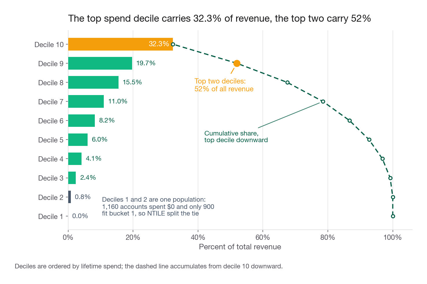
The top tenth carries 32.3 percent of revenue and the top fifth 52 percent, which is the sentence a PM writes down.
Now the first bite. Decile 1 holds 900 accounts that spent zero, and decile 2's minimum is also zero, because 1,160 accounts spent nothing and only 900 fit the first bucket. NTILE splits identical values across boundaries wherever it must, so 260 accounts behaving exactly like decile 1 get labelled decile 2. Send decile 2 a winback offer and skip decile 1 and you have split an identical population on nothing.
The second bite is arithmetic: NTILE gives equal sizes only when the row count divides evenly. Inside New Zealand's 353 accounts it yields three buckets of 36 and seven of 35, larger first. The tie-safe alternative is CUME_DIST, which gives every row with the same value the same answer:
| orders | accounts | cume_dist |
|---|---|---|
| 0 | 162 | 0.1306 |
| 1 | 166 | 0.2645 |
| 2 | 149 | 0.3847 |
Every UK account with zero orders sits at 0.1306, no exceptions. If a segment definition must be reproducible, threshold on CUME_DIST rather than an NTILE label.
Top three per country
This is the top-N-per-group shape from the previous lesson, with the partition changed to country and the sort to spend DESC, user_id. One thing about the base CTE still matters: build per-account spend with a LEFT JOIN and COALESCE(SUM(amount_usd), 0) so never-buyers stay at zero rather than disappearing, which counts if that CTE later feeds a decile. It returns account 3002 at 1,632.04 in the UK and 3005 at 1,226.35 in New Zealand.
Interview tip: Before writing NTILE, ask whether the underlying values have many ties. Integer counts almost always do, and NTILE on a tied column produces segments nobody can reproduce from the data alone.
Common traps
Reading a censored cohort cell. The newest cohort's later weeks are partial numerators over full denominators. Fix: floor-divide each cohort's minimum days observed by the period length and blank every later cell.
Comparing "ever did X" across cohorts. Older cohorts had more time. Fix: rewrite as "did X within N days of signup", N small enough for the youngest.
Casting a day difference to an integer to bucket it. Several engines round rather than truncate, so day four lands in week one. Fix:
FLOOR(days / 7.0), then check week zero is the largest bucket.Bare UNION between two period exports. It deduplicates identical rows, and identical rows are real. Fix:
UNION ALL.Omitting the frame clause on an ordered window. The default
RANGEgives every same-day row the same running total. Fix: writeROWS BETWEEN UNBOUNDED PRECEDING AND CURRENT ROWevery time.Accumulating over raw rows when the question says "per day", or without PARTITION BY. Two baskets on one date give two rows, and a missing partition leaks the total across accounts. Fix: aggregate to the requested grain, partition, then check the second account's first row equals its own first value.
Filtering in the same select as the window. It sees only surviving rows, so trailing averages and cumulative sums silently restart. Fix: window in a CTE, filter outside it.
Scaling partial-period revenue by day count. Weekends and weekdays are not worth the same. Fix: reweight by the calendar, or extrapolate only from whole weeks.
ROW_NUMBER when ties must survive, or RANK when the row count is fixed. Fix: choose from intent, and give ROW_NUMBER a tie-break column so reruns match.
Trusting NTILE labels on a tied column. Identical values land in different buckets. Fix: use CUME_DIST when the segment must be reproducible.
Quick self-check
Answer these out loud, in full sentences, the way you would in the room.
Your newest cohort drops from 53 percent to 0.5 percent across five weeks. What do you say first, and what calculation decides which cells you may interpret?
"Power user means ten purchases." Give the two readings, say how far apart they land when baskets average five items, and which you would push for.
Write the running total of daily spend per account. State the partition, the order, and the frame, then say what changes if you drop the frame and two orders share a date.
It is the 12th of a 30 day month and revenue to date is 219,337 dollars. Give the naive forecast, say whether it is high or low, and name the calendar fact that decides the direction.
Build a median without a percentile function. Explain why the surviving-row test uses "within one" rather than equality, and what happens on an even count.
Three customers tie for seventh. For each of ROW_NUMBER, RANK, and DENSE_RANK, say how many rows a
<= 8filter returns and name a requirement making each one correct.