5.1 When You Cannot Randomize Users
Find the core decision, design, or behavior signal.
Turn the lesson into a concise response blueprint.
Name the trap you would avoid in a real interview.
Use these checkpoints as your reading path before diving into the full lesson.
- 1Why this matters in interviews
- 2The interference test you run before an...
- 3Push the treatment to its limits
- 4Three mechanisms, three different fixes
- 5Choosing the randomization unit
Some products cannot be tested by flipping a coin per user, and an interviewer who asks you to test one is checking whether you notice. This lesson gives you the check that catches those products in the first minute, the menu of designs that replace user randomization, and the arithmetic that tells you what each replacement actually costs. The decision it helps you make is which unit to randomize on, and what evidence you will accept from a design that is far weaker than the one you wanted.
Why this matters in interviews
The previous lesson covered randomization done properly: the unit, the hash, the balance checks, the ways assignment leaks. This one starts one step earlier, at the question of whether user-level randomization is legal at all for the product in front of you.
Two things get scored here, and they are scored in order.
The first is whether you notice. A candidate who hears "a courier marketplace is shipping a new dispatch algorithm" and immediately says "split couriers fifty-fifty, run a two-sample t-test on trips per courier" has failed before saying anything about statistics. Every downstream detail can be correct and the answer is still wrong, because treating one courier changed the outcome for the courier who did not get the treatment. Interviewers use marketplaces, social products, and ad auctions precisely because the trap is invisible if you are pattern-matching to a template.
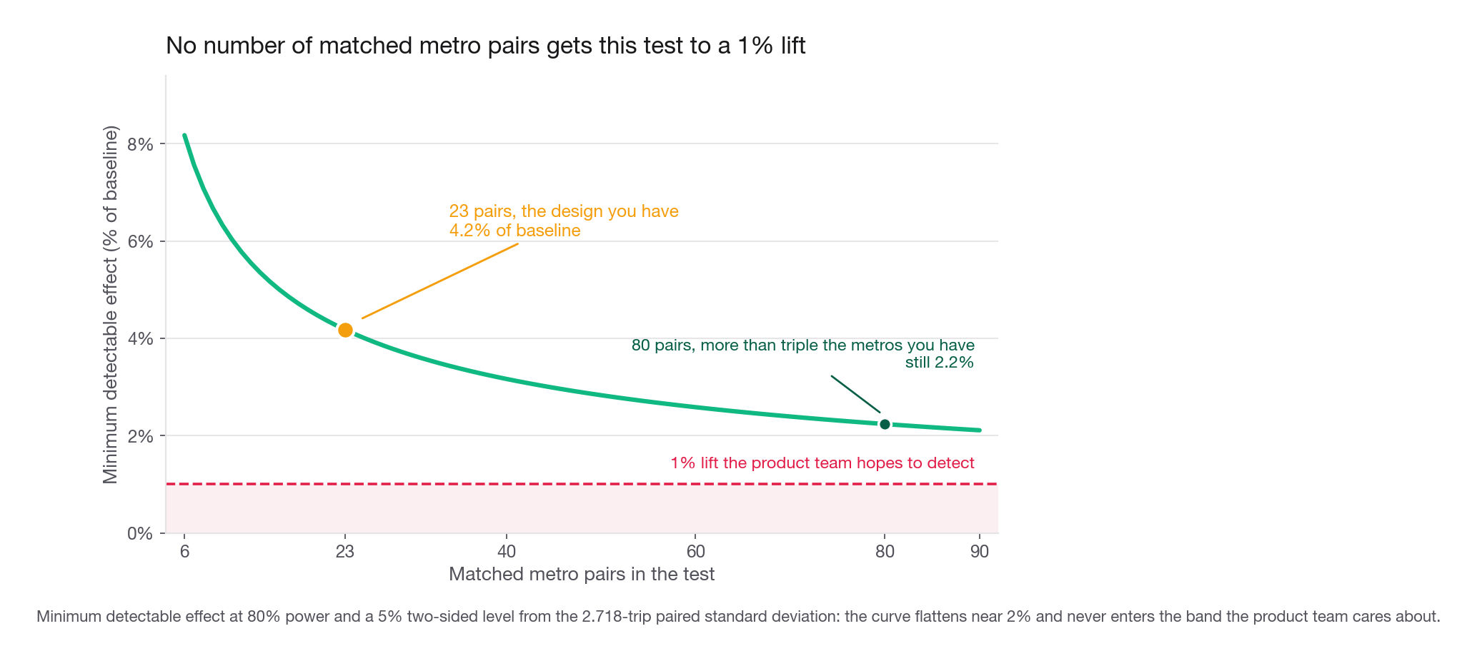
The second is whether you can price the alternative. Noticing the problem is table stakes at senior level. What separates candidates is the next sentence. Weak: "so we would test by market instead." That is a label, not a design. Strong: "so we would test by metro, which leaves us roughly twenty-three pairs, which puts our minimum detectable effect near four percent, so this design can only adjudicate changes we expect to be large; if the product team believes the lift is one percent, I would tell them this test cannot answer the question and propose something else."
That second answer is the lesson compressed: detect the interference, choose a unit, price the unit, then say whether the resulting evidence can carry the decision.
Interview tip: The sentence that marks you as senior is not "we cannot randomize users." It is "here is the minimum detectable effect this design gives us, and here is whether that is good enough for the decision."
The interference test you run before anything else
User-level tests rest on an assumption with a formal name, stable unit treatment value assumption, and a plain-language version worth memorizing: one user's outcome depends on that user's own assignment and on nothing else. When it fails, the control group is contaminated by the treatment, and the comparison measures something other than what you wanted.
Push the treatment to its limits
You do not need a theory of the product to detect interference, only a thirty-second thought experiment, because interference is a property of the mechanism rather than of the effect size. Imagine the treatment is so broken that treated users cannot use the product at all, and ask whether anything about the control group's experience changes. Then imagine it is so good that treated users triple their usage, and ask again.
Run it on Tramline, a fictional same-day courier marketplace operating in forty-six metros with about 220,000 active couriers. The change under test is a redesigned offer card that helps couriers pick better batches. If half the couriers in Denver get an offer card so broken they stop accepting batches, the other half of Denver's couriers see a flood of unclaimed orders and their trips per week go up. If the offer card is fantastic and treated couriers sweep the board, control couriers get the leftovers and their trips go down. Both directions move the control group. There is no user-level test here.
Run it on Kettle, the meal planning app from the metrics section. If half of Kettle's users get a broken recipe importer, does the other half's cooking behavior change? No. Users do not compete for recipes and do not see each other. User-level randomization is fine.
The probe costs nothing and is the highest-leverage habit in this section.
Three mechanisms, three different fixes
Interference is not one thing. Naming the mechanism matters because the mechanism determines both the direction of the bias and which alternative design fixes it.
| Mechanism | What is shared | Typical products | Bias in a naive user split | Design that fixes it |
|---|---|---|---|---|
| Congestion or competition | A finite pool of demand, supply, or attention | Courier and rideshare marketplaces, ticketing, ad auctions | Overstates: treatment wins by taking share from control | Randomize the market, or switch back in time |
| Contagion or transmission | Content, invitations, and social signals flowing between users | Social feeds, messaging, referral loops, multiplayer | Understates: control is lifted by treated neighbors | Randomize graph clusters, or run a saturation design |
| Shared machinery | A model, a budget, a cache, a queue, or a rate limit | Ranking systems, bid pacing, notification budgets, ML retraining | Either direction, and often unstable over the run | Isolate the shared resource per arm, or randomize the resource |
The third row is the one candidates almost never mention and interviewers love. If the treatment arm's clicks feed the same ranking model that serves control, the arms are training each other and the effect drifts across the run. Same with a shared daily send budget: a treatment that sends more notifications is starving control rather than being compared against the status quo.
Interview tip: Name the mechanism, not just the word "interference." Congestion, contagion, and shared machinery lead to three different designs, and the interviewer wants to see you pick.
Choosing the randomization unit
Once user-level is off the table, you are choosing a coarser unit. Every step up the ladder buys independence and pays for it in statistical power, because the number of units collapses far faster than the number of users does.
| Unit | Independent enough when | Units you realistically have | What it costs | Watch out for |
|---|---|---|---|---|
| User | No shared resource, no social graph edge | Hundreds of thousands | Nothing, this is the best case | Multi-device users breaking the hash |
| Household or device cluster | Interference is confined to co-located people | Tens of thousands | Small variance increase | Households of size one dominate |
| Account or team | Interference is inside an org boundary | Hundreds to low thousands | Large accounts dominate the average | Weighting by seats versus by account |
| Graph cluster | Most edges stay inside a cluster | Thousands, but very uneven | Leakage on cut edges | Cluster sizes with heavy tails |
| Metro or market | Users in different cities do not interact | Tens | Severe, this is the expensive one | External shocks hitting one market |
| Time slice, switchback | Carryover between periods decays fast | Hundreds of periods | Carryover bias, autocorrelation | Effects with long memory |
The rule is not "use the smallest unit." It is: use the smallest unit for which the extreme-case probe comes back clean, then be honest about the power it leaves you.
A panel to make this concrete
Everything below runs on a synthetic metro-week panel for Tramline with the schema described: forty-six metros, twenty-six weeks, thirteen before the switch and thirteen after, one row per metro per week. The outcome is completed deliveries per active courier per week. This block builds it deterministically, including a matched-pair assignment on the pre-period level and a true treatment effect of 1.55 trips, about 4.1 percent of the 38.0 baseline.
import numpy as np
import pandas as pd

SEED = 51074
rng = np.random.default_rng(SEED)

N_METRO, N_WEEK, TRUE_LIFT = 46, 26, 1.55
metros = np.array([f"metro_{i:02d}" for i in range(1, N_METRO + 1)])
base = rng.normal(38.0, 6.5, N_METRO)      # baseline trips per active courier
drift = rng.normal(0.0, 0.09, N_METRO)     # metro specific weekly trend
couriers = rng.integers(900, 14000, N_METRO)

order = np.argsort(base)                   # matched pairs on baseline level
treated, pair_id = np.zeros(N_METRO, int), np.zeros(N_METRO, int)
for k in range(0, N_METRO, 2):
    a, b = order[k], order[k + 1]
    pair_id[a] = pair_id[b] = k // 2
    treated[a if rng.random() < 0.5 else b] = 1

week = np.arange(1, N_WEEK + 1)
season = 1.1 * np.sin(2 * np.pi * week / 13.0)
frames = []
for i in range(N_METRO):
    lift = TRUE_LIFT * treated[i] * (week > 13)
    frames.append(pd.DataFrame({
        "metro": metros[i], "week": week, "pair_id": pair_id[i],
        "couriers": couriers[i], "treated": treated[i],
        "post": (week > 13).astype(int),
        "trips_per_courier": base[i] + drift[i] * week + season
                             + rng.normal(0, 3.4, N_WEEK) + lift,
    }))
panel = pd.concat(frames, ignore_index=True)
print(panel.shape, panel["treated"].sum() // N_WEEK)
(1196, 7) 23Twenty-three treated metros, twenty-three controls, 1,196 rows. Note what that count implies: 220,000 couriers become 1,196 observations, and after collapsing to one pre-post change per metro, forty-six. That collapse is the whole story.
What randomizing by metro actually costs you
Start with the number, because the number is what wins the interview.
A user-level test on Tramline would have 110,000 couriers per arm. With a weekly standard deviation near 14 trips, the minimum detectable effect at eighty percent power and a five percent two-sided level is roughly 0.17 trips, about 0.44 percent of baseline. The metro-level design, computed below, lands near 4.2 percent: nine and a half times worse on the effect scale and about ninety times worse on the variance scale. Forty-six metros holding 220,000 couriers buy the statistical information of roughly 2,400 independently randomized couriers. Ninety-nine percent of your data is spent purchasing independence, and saying so reframes the conversation from "which test do I run" to "is this decision worth the only valid design."
There is a second reason to accept that cost, and it is not about validity. A user-level test estimates the direct effect on a treated courier with every other courier's assignment held fixed. A metro-level test estimates the total effect of treating the whole metro, direct effect plus the spillover inside it, which is the quantity the launch decision needs. You are not buying a cleaner version of the same number, you are buying a different and more relevant one. Effects that cross metro boundaries, national supply, brand, a shared ad budget, sit outside even this design.
Three estimators, three very different confidence intervals
Collapse the panel to one pre mean and one post mean per metro, then compare estimators on identical data.
cell = (panel.groupby(["metro", "pair_id", "treated", "post"])["trips_per_courier"]
             .mean().unstack("post"))
cell.columns = ["pre", "post"]
cell = cell.reset_index()
cell["change"] = cell["post"] - cell["pre"]

def gap(col):
    a = cell.loc[cell.treated == 1, col].to_numpy()
    b = cell.loc[cell.treated == 0, col].to_numpy()
    est = a.mean() - b.mean()
    se = np.sqrt(a.var(ddof=1) / len(a) + b.var(ddof=1) / len(b))
    return est, se

for col, label in [("post", "post-period levels"), ("change", "per-metro change")]:
    e, s = gap(col)
    print(f"{label:20s} est={e:6.3f} se={s:5.3f} ci=[{e - 1.96 * s:6.3f},{e + 1.96 * s:6.3f}]")
post-period levels est= 1.633 se=2.555 ci=[-3.375, 6.640]
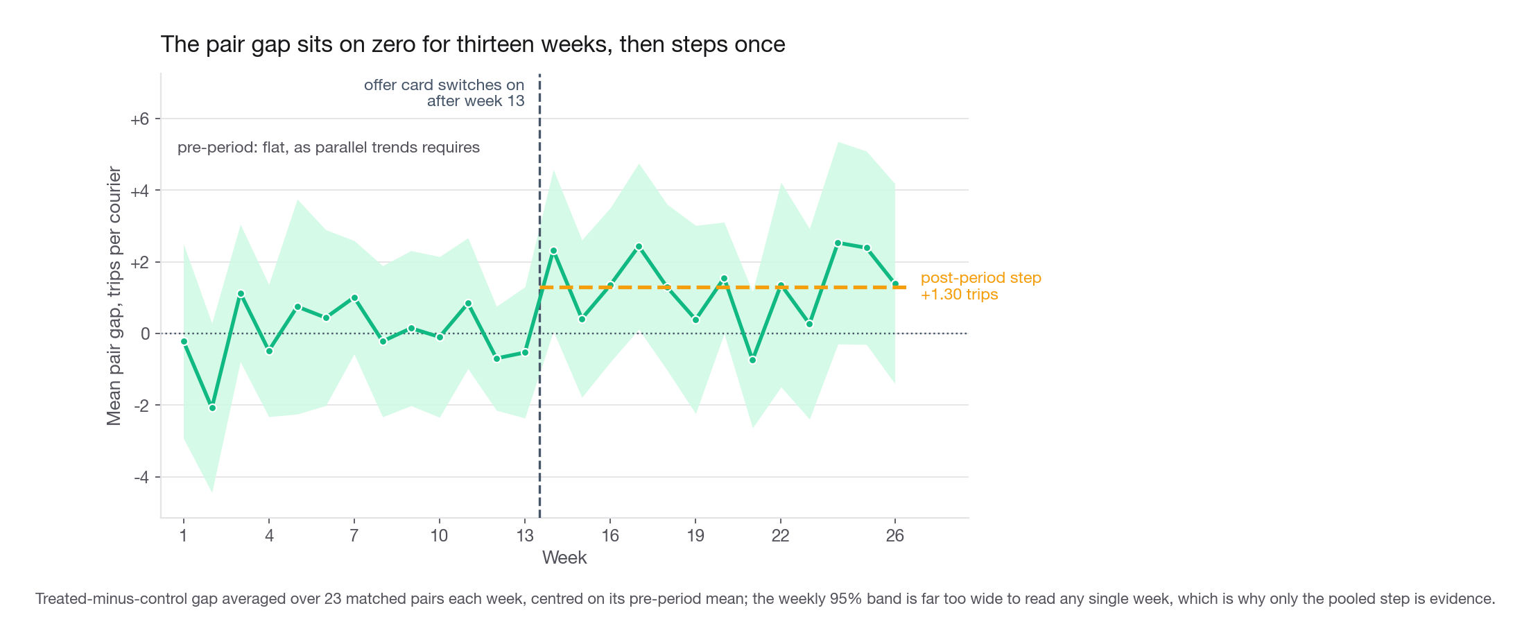
per-metro change est= 1.303 se=0.566 ci=[ 0.194, 2.412]Both point estimates sit near the truth of 1.55. They are not remotely equivalent. Comparing post-period levels carries all of the between-metro variation, standard deviation 6.5 trips, so its interval spans minus nine percent to plus seventeen percent and cannot distinguish a disaster from a triumph. Differencing each metro against its own pre-period removes its level entirely and shrinks the standard error by a factor of four and a half. That is the practical case for difference-in-differences, and it is a variance argument before it is a causal one: you are removing the nuisance variance of "Denver is simply busier than Tucson."
The number that ends the argument
Now use the pair structure and compute the minimum detectable effect the design can support.
w = cell.pivot(index="pair_id", columns="treated", values="change")
d = (w[1] - w[0]).to_numpy()
est, sd = d.mean(), d.std(ddof=1)
se = sd / np.sqrt(len(d))
print(f"paired DiD est={est:.3f} se={se:.3f} pairs={len(d)} pair sd={sd:.3f}")

perm_rng = np.random.default_rng(7)
signs = perm_rng.choice([-1.0, 1.0], size=(40000, len(d)))
null = (signs * d).mean(axis=1)
print("permutation p:", round((np.abs(null) >= abs(est)).mean(), 4))

for n_pairs in (10, 23, 40, 80):
    mde = 2.80 * sd / np.sqrt(n_pairs)
    print(f"{n_pairs:3d} pairs -> mde {mde:5.3f} trips = {100 * mde / 38.0:4.2f}% of baseline")
paired DiD est=1.303 se=0.567 pairs=23 pair sd=2.718
permutation p: 0.0308
10 pairs -> mde 2.406 trips = 6.33% of baseline
23 pairs -> mde 1.587 trips = 4.18% of baseline
40 pairs -> mde 1.203 trips = 3.17% of baseline
80 pairs -> mde 0.851 trips = 2.24% of baselineThree things to take from this output.
The permutation test is the right inference and trivial to run. Under the null that assignment within a pair was arbitrary, flipping the sign of any pair's difference yields an equally likely dataset, so forty thousand random sign flips give the null distribution directly. With twenty-three pairs, do not lean on a t distribution and a normality assumption you cannot check.
The paired standard error, 0.567, is identical to the unpaired one, 0.566. Pairing bought nothing, and that is the lesson rather than a bug: these pairs were matched on baseline level, and differencing already removes baseline level. Matching on a feature the estimator absorbs anyway is theatre.
The last table is what you bring to the product team. Even eighty pairs, which is 160 metros and more than three times the footprint Tramline actually operates, only reaches 2.2 percent, so no version of this design adjudicates a one percent change. If the honest prior on the offer card is one percent, the recommendation is to not run the market test at all.
Interview tip: Bring a minimum detectable effect to every market-test answer. "About twenty pairs, so roughly four percent" is a complete thought; "we would test by market" is half of one.
Matched-market design done properly
Matching is a design step, done before any treatment exists, on pre-period data only. Doing it after you see outcomes is how you talk yourself into a result.
Match on trajectory, if the trajectory is measurable
The estimator differences away the level. What it cannot difference away is a market whose trend was already diverging, so the obvious next move is to add pre-period slope to the matching features. Treat that as a hypothesis rather than a rule, because whether it earns anything depends on whether a slope is estimable at all from the pre-period you have.
pre = panel[panel.week <= 13].pivot(index="week", columns="metro",
                                    values="trips_per_courier")
level = pre.mean()
slope = pre.apply(lambda s: np.polyfit(pre.index, s, 1)[0])
z = lambda s: (s - s.mean()) / s.std(ddof=0)
feat = pd.DataFrame({"level": z(level), "slope": z(slope)})

names = list(feat.index)
F = feat.to_numpy()
dist = pd.DataFrame(np.sqrt(((F[:, None, :] - F[None, :, :]) ** 2).sum(-1)),
                    index=names, columns=names)
np.fill_diagonal(dist.values, np.inf)

remaining, proposed = set(names), []
while remaining:
    sub = dist.loc[list(remaining), list(remaining)]
    i, j = np.unravel_index(np.argmin(sub.to_numpy()), sub.shape)
    proposed.append((sub.index[i], sub.columns[j], round(sub.iloc[i, j], 3)))
    remaining -= {sub.index[i], sub.columns[j]}

truth = {frozenset(g["metro"]) for _, g in panel.groupby("pair_id")}
print("pairs:", len(proposed), "worst distance:", max(p[2] for p in proposed))
print("agree with the level-only pairing:", sum(frozenset(p[:2]) in truth for p in proposed))
pairs: 23 worst distance: 1.778
agree with the level-only pairing: 2Two of twenty-three. Resist the reading that this proves slope is the better feature. Adding any second dimension scrambles a partition that was built by sorting on one, and a slope made of pure noise would scramble it just as thoroughly. The only thing that settles it is the check you are about to write into your own plan: does the new pairing actually shrink the pair difference?
counter = (cell.set_index("metro")["change"]
           - TRUE_LIFT * cell.set_index("metro")["treated"])   # strip the known lift

def pair_spread(pairs):
    diff = np.array([counter[a] - counter[b] for a, b in pairs])
    return float(np.sqrt((diff ** 2).mean()))     # orientation free

level_pairs = [tuple(g["metro"].unique()) for _, g in panel.groupby("pair_id")]
slope_pairs = [(a, b) for a, b, _ in proposed]
for name, prs in [("level only", level_pairs), ("level + slope", slope_pairs)]:
    sp = pair_spread(prs)
    print(f"{name:13s} pair spread {sp:.3f}  ->  mde at 23 pairs "
          f"{100 * 2.80 * sp / np.sqrt(23) / 38.0:4.2f}% of baseline")

sxx = ((np.arange(1, 14) - 7.0) ** 2).sum()
print(f"slope se {3.4 / np.sqrt(sxx):.3f} vs true drift sd 0.09  ->  "
      f"reliability {0.09 ** 2 / (0.09 ** 2 + 3.4 ** 2 / sxx):.3f}")
level only pair spread 2.669 -> mde at 23 pairs 4.10% of baseline
level + slope pair spread 2.829 -> mde at 23 pairs 4.35% of baseline
slope se 0.252 vs true drift sd 0.09 -> reliability 0.113It does not shrink it. The pairing this section just recommended is slightly worse on its own panel, and the last printed line says why. A slope fitted to thirteen weekly points with residual standard deviation 3.4 carries a standard error of 0.252, against a true spread of metro trends of 0.09. By variance that estimate is about eighty-nine percent noise, a reliability of 0.113, so the matcher is mostly pairing markets on their measurement error. The ceiling follows without any simulation: a pair difference here is thirteen weeks of drift gap plus two sample means of weekly noise, so a random pairing sits at 2.509, a perfect match on a slope estimate this noisy can reach only 2.446, and a perfect match on the true drifts would reach 1.886. Slope matching is fighting for two and a half percent of a twenty-five percent opportunity, and four hundred fresh draws of the generator agree on the ordering: 2.463 unpaired, 2.460 level-matched, 2.423 with level and slope, 1.883 with the true drift.
The transferable lesson is one comparison, run before any matcher. Put the standard error of the trend you want to match on next to the spread of that trend across markets. If the standard error dominates, trend matching is theatre for exactly the reason level matching was, and the senior move is to say so rather than ship the pairing. Shrinking the slope does not rescue it, since a linear shrinkage is monotone and returns the identical pairing. A longer pre-period would: this generator needs about twenty-six weeks before the slope reaches coin-flip reliability and about forty-one before it reaches eighty percent, because a slope's information grows with the cube of the window. That is a budget conversation, not a line of code.
The greedy loop always returns a complete pairing, and it will happily marry the last two leftovers at a distance of 1.778 standard deviations, which is not a pair in any meaningful sense. Set a distance ceiling, drop the metros that exceed it, and run twenty pairs instead of twenty-three. Losing three pairs costs about seven percent of your precision; keeping a fraudulent pair costs the credibility of the test.
The balance metric that is not your outcome
Matching on the outcome's history is necessary and insufficient, because two markets can share a trips history and still diverge during the run for unrelated reasons. So you pick a second series the treatment has no plausible path to affect, and watch it throughout.
For a courier-side offer card, that series is merchant-side: new merchant signups per week. The offer card changes how couriers choose among batches; it does not change whether a bakery in Portland joins. If signups track between paired metros for thirteen weeks and then split in week nineteen, something happened in that metro that has nothing to do with you, and the pair is contaminated. Pick the series before the run and write it into the plan. Picking it afterward, once you dislike the result, is not a robustness check.
Interview tip: When you describe a matched-market design, name the placebo series out loud. It is the cheapest signal that you have run one of these rather than read about one.
Difference-in-differences and the assumption you must defend
The paired computation above is difference-in-differences with an unusually clean structure. The general form uses a regression with a fixed effect for each metro and a fixed effect for each week, plus a single indicator for treated metros in the post period. The metro effects absorb permanent differences between markets, the week effects absorb anything hitting the whole country in a given week, and the interaction is your estimate.
The part interviewers probe is the standard error. Trips per courier in Denver this week is correlated with the same figure last week, so 1,196 rows are nothing like 1,196 independent observations, and treating them as independent produces a confident, wrong interval.
def twfe(df, outcome="trips_per_courier"):
    y = df[outcome].to_numpy()
    D = (df["treated"] * df["post"]).to_numpy().reshape(-1, 1).astype(float)
    FE = pd.get_dummies(df[["metro", "week"]].astype(str), drop_first=True).to_numpy(float)
    X = np.hstack([np.ones((len(df), 1)), D, FE])
    beta = np.linalg.pinv(X) @ y
    resid = y - X @ beta
    bread = np.linalg.pinv(X.T @ X)
    meat = np.zeros((X.shape[1], X.shape[1]))
    for _, idx in df.groupby("metro").indices.items():
        s = X[idx].T @ resid[idx]
        meat += np.outer(s, s)
    G = df["metro"].nunique()
    V = bread @ (G / (G - 1.0) * meat) @ bread
    iid = (resid @ resid / (len(y) - np.linalg.matrix_rank(X))) * bread
    return beta[1], np.sqrt(V[1, 1]), np.sqrt(iid[1, 1])

b, se_cl, se_iid = twfe(panel)
print(f"est={b:.3f}  clustered se={se_cl:.3f}  iid se={se_iid:.3f}  t={b / se_cl:.2f}")
est=1.303 clustered se=0.559 iid se=0.403 t=2.33The independence-assuming standard error is thirty-nine percent too small, which would turn a t of 2.33 into a t of 3.23 and a marginal result into a confident one. Cluster on the unit of randomization, always, and say the word "cluster" in the interview because it is a fast credibility signal.
One caveat worth volunteering: cluster-robust standard errors are themselves asymptotic in the number of clusters, and forty-six is not comfortably large. Below roughly forty clusters, prefer the permutation test from earlier or a wild cluster bootstrap. Notice that this is a second, independent reason the permutation test is the better default at this scale.
Testing parallel trends instead of asserting it
Difference-in-differences is unbiased only if the two groups would have moved together absent the treatment. That is a counterfactual and cannot be verified. What you can do is check the period where you know the treatment was absent.
placebo = panel[panel.week <= 13].copy()
placebo["post"] = (placebo["week"] > 7).astype(int)   # a switch date that never happened
pc = (placebo.groupby(["pair_id", "treated", "post"])["trips_per_courier"]
             .mean().unstack("post"))
pc.columns = ["a", "b"]
pc = pc.reset_index()
pc["change"] = pc["b"] - pc["a"]
pw = pc.pivot(index="pair_id", columns="treated", values="change")
pd_ = (pw[1] - pw[0]).to_numpy()
print(f"placebo est={pd_.mean():.3f} se={pd_.std(ddof=1) / np.sqrt(len(pd_)):.3f} "
      f"t={pd_.mean() / (pd_.std(ddof=1) / np.sqrt(len(pd_))):.2f}")
placebo est=-0.172 se=0.531 t=-0.32A fake switch in the middle of the pre-period produces an estimate indistinguishable from zero. That is the reassurance you want, and its absence is disqualifying: if a treatment that had not happened yet produces a significant effect, your design is measuring divergence, not causation.
Two refinements if the interviewer pushes. Plot the pair-level gap week by week instead of collapsing to two averages, so a reader can see whether the gap was flat before the switch and stepped after. And note that a placebo test has power too: with twenty-three pairs it only detects a pre-trend of about four percent, so a null placebo fails to reject a generous null rather than proving parallel trends.
Synthetic control, and when it is theatre
Sometimes you get one treated market, not twenty-three: a regulator approves the change in a single state, or ops can only staff one city. Synthetic control is the standard answer. Build a weighted blend of untreated markets that reproduces the treated market's pre-period series, then read the post-period gap between the real unit and its synthetic twin. The weights are non-negative and roughly sum to one, which keeps the synthetic unit inside the range of observed markets and blocks the extrapolation unconstrained regression would happily do.
from scipy.optimize import nnls

wide = panel.pivot(index="week", columns="metro", values="trips_per_courier")
donors = list(panel.loc[panel.treated == 0, "metro"].unique())
focus = panel.loc[panel.treated == 1, "metro"].unique()[0]

def synth(target, pool):
    A = np.vstack([wide.loc[1:13, pool].to_numpy(), 10 * np.ones(len(pool))])
    b_ = np.append(wide.loc[1:13, target].to_numpy(), 10.0)   # soft sum-to-one
    weights, _ = nnls(A, b_)
    fitted = wide[pool].to_numpy() @ weights
    pre_rmse = np.sqrt(np.mean((wide.loc[1:13, target].to_numpy() - fitted[:13]) ** 2))
    post_rmse = np.sqrt(np.mean((wide.loc[14:26, target].to_numpy() - fitted[13:]) ** 2))
    gap = (wide.loc[14:26, target].to_numpy() - fitted[13:]).mean()
    return weights, pre_rmse, post_rmse, gap

w_, pre_rmse, post_rmse, gap = synth(focus, donors)
print(f"{focus}: pre rmse={pre_rmse:.3f} post gap={gap:.3f} ratio={post_rmse / pre_rmse:.2f}")
print("donors used:", int((w_ > 1e-6).sum()), "sum of weights:", round(w_.sum(), 3))
metro_01: pre rmse=2.573 post gap=-0.025 ratio=1.84
donors used: 6 sum of weights: 1.037The true effect in this metro is plus 1.55 trips. The synthetic control estimate is minus 0.025. It found nothing.
This is not a failure of the code, and it is the most useful result on this page. Look at the pre-period fit: a root mean squared error of 2.573 trips against a target effect of 1.55. The twin cannot track the real metro to better than 2.6 trips in a stretch where the true gap is exactly zero, so it has no chance of resolving 1.55 afterward.
You can make that precise. The post-period gap averages thirteen weeks of noise from the treated metro plus a weighted blend from six donors. With a weekly standard deviation of 3.4 and weights whose squares sum to 0.254, the standard error of the mean gap is about 1.06 trips, so the single-metro minimum detectable effect is near 3.0 trips, or 7.8 percent, twice as blunt as the twenty-three-pair test.
Inference here is placebo-in-space: refit treating each untreated market in turn as if it had been treated, collect the ratio of post-period to pre-period fit error, and see where the real treated unit ranks. It ranks twelfth of twenty-four, a rank-based p-value of 0.50.
| Situation | Reach for | Why |
|---|---|---|
| Twenty or more markets, half treated | Matched-pair difference-in-differences with a permutation test | Uses every unit, the inference needs no distributional assumption |
| One treated market, a large expected effect, a smooth outcome | Synthetic control with placebo-in-space inference | Only method that builds a credible counterfactual from one unit |
| One treated market, a small expected effect, a noisy weekly outcome | Nothing, and say so | Pre-period fit error already exceeds the effect you are hunting |
| A few treated markets, one shared shock | Pooled synthetic control on the aggregate treated series | Averaging treated units first cuts the noise before you fit |
| No pre-period at all | Nothing, wait for one | Every method on this page is a pre-period method |
The row that earns points is the third. Reaching for a fancier estimator when the data is too noisy for a simple one shows you think estimators create information. Compare pre-period fit error to the target effect before fitting anything, and be willing to conclude the study is not worth running.
Interview tip: Report the pre-period fit error next to the effect you hope to detect. If the fit error is larger, say the design cannot answer the question instead of producing a number.
Switchbacks: randomize time instead of people
When the mechanism is congestion and it clears fast, one design recovers most of the lost power: split time instead of couriers or metros. Denver runs the new dispatch logic from 09:00 to 09:30, the old from 09:30 to 10:00, with the order randomized. Every metro contributes both arms, so between-metro variance vanishes and the unit count becomes periods rather than cities.
The cost is carryover. A batch offered at 09:29 under the new logic is often still moving at 09:35, so the opening minutes of each control period are contaminated. Standard practice is to discard a burn-in window sized to roughly the ninetieth percentile of the effect's decay time, and to cluster standard errors by day.
| Design axis | Matched markets | Switchback |
|---|---|---|
| Effective unit count | 20 to 50 markets | 200 to 2,000 periods |
| Removes between-market variance | Only by differencing | Yes, structurally |
| Main threat | An external shock in one market | Carryover across period boundaries |
| Works when the effect is slow | Yes | No, carryover swamps it |
| Ops burden | Low, one flag per market | High, needs reliable scheduled flips |
| Reasonable metric | Weekly trips, weekly earnings | Wait time, accept rate, per-batch cost |
The dividing line is memory. Dispatch matching acts within minutes, so switchbacks are excellent. A pay-structure change alters behavior for weeks, so switchbacks are useless because the treatment period never truly ends. Ask for the decay time; if it exceeds a plausible period length, you are back to markets.
Network effects: which way does the bias run
Now the second half of the lesson, and the part candidates most often get backwards.
Take Thicket, a fictional social app for home gardeners. The team ships a composer that makes posting easier, gives it to a random half of users, and measures likes given per user per week. Treatment wins by a healthy margin. The interviewer asks: after rolling out to everyone, will the metric rise by that same margin, more, or less?
The instinct is "the same," because that is what an experiment is supposed to tell you. The correct answer is "more," because the control group was never a picture of the untreated world.
Two channels push the same way. Contamination of control: a treated gardener posts more, their untreated followers see more posts, and those untreated users give more likes than they would have with no treatment anywhere, so the measured gap understates. And compounding at full scale: once everyone has the composer, everyone's followers are posting more too, and the extra supply feeds back into demand. Both effects only fully exist in a world the experiment never created.
net_rng = np.random.default_rng(3141)
N, DEG, UPLIFT = 20_000, 9, 0.12
src = net_rng.integers(0, N, N * DEG // 2)
dst = net_rng.integers(0, N, N * DEG // 2)
base_posts = net_rng.gamma(2.0, 1.4, N)      # weekly posts if untreated

def likes_given(T):
    posts = base_posts * (1 + UPLIFT * T)    # own composer effect on supply
    feed = np.zeros(N)
    np.add.at(feed, src, posts[dst])         # supply reaching each user's feed
    np.add.at(feed, dst, posts[src])
    return 0.31 * feed * (1 + UPLIFT * T)    # own composer effect on liking

T = (net_rng.random(N) < 0.5).astype(float)
L = likes_given(T)
measured = L[T == 1].mean() / L[T == 0].mean() - 1
true_lift = likes_given(np.ones(N)).mean() / likes_given(np.zeros(N)).mean() - 1
print(f"measured A/B lift {100 * measured:.2f}%   true full-rollout lift {100 * true_lift:.2f}%")
print(f"understatement factor {true_lift / measured:.2f}")
measured A/B lift 11.34% true full-rollout lift 25.44%
understatement factor 2.24The experiment reports eleven percent; the truth at full rollout is twenty-five. A team that trusts the arm gap under-invests in a feature worth more than double what it measured, and builds a quarterly forecast the product then blows past, which quietly erodes trust in the experimentation platform.
And now the opposite sign
Do not walk away with the rule "spillover means we understate." It depends entirely on whether the treatment creates value or moves it around.
mk_rng = np.random.default_rng(2718)
M, ORDERS, LIFT = 4_000, 150_000, 0.10
appeal = mk_rng.lognormal(0.0, 0.45, M)      # baseline chance of winning a batch
Tm = (mk_rng.random(M) < 0.5).astype(float)

def trips(t):
    share = appeal * (1 + LIFT * t)
    return ORDERS * share / share.sum()      # a fixed pool of orders, split

ab = trips(Tm)
print(f"measured lift {100 * (ab[Tm == 1].mean() / ab[Tm == 0].mean() - 1):.2f}%")
print(f"true full-rollout lift {100 * (trips(np.ones(M)).mean() / trips(np.zeros(M)).mean() - 1):.2f}%")
measured lift 10.59%
true full-rollout lift 0.00%Here the offer card is purely redistributive. Orders in the metro are fixed, so a courier who wins more batches wins them from another courier. The experiment reports a ten and a half percent lift with a tiny p-value and the true effect of shipping to everyone is zero. This is the failure that ships bad features, because the measured result is large, clean, and completely spurious.
This is also the cleanest argument for the metro design. Run the same offer card as a market test and every courier in a treated metro gets it, so the fixed pool of orders is split among couriers who are all better at claiming them, and trips per courier comes back essentially unchanged, roughly the true zero, which is the right answer. The ninety-fold power penalty bought the only number the launch decision could use. Say roughly, because the exact zero is an artifact of a fixed order pool: give demand any elasticity and a market test returns the small genuine value creation instead.
| Mechanism | Direction of naive bias | Concrete tell | What to say |
|---|---|---|---|
| Contagion through a feed or graph | Understates the true effect | Treated users' neighbors move too | Expect full rollout to beat the arm gap |
| Zero-sum competition for supply or demand | Overstates, sometimes entirely | Control's metric falls while treatment rises | The gap may be pure redistribution |
| Shared budget or rate limit | Overstates | Control's volume drops with no product change | Give each arm its own budget before trusting anything |
| Shared model retrained on both arms | Drifts over the run | Effect grows or shrinks monotonically week to week | Freeze the model or train one per arm |
| Reciprocity, messaging and invites | Understates | Control replies to treated users' messages | Randomize by connected component |
The diagnostic that distinguishes contagion from competition takes one query, and it is the strongest thing you can say here: plot the control arm's absolute metric against the same metric in the same weeks last year, or against a holdout population that was never eligible. If control is above its own historical baseline, treatment is lifting it and you are understating. If control is below, treatment is stealing from it and you are overstating. The arm gap alone can never tell you which world you are in.
Interview tip: Never analyze only the gap between arms. Always look at the control arm's absolute level against an untouched baseline, because that single line tells you the sign of your spillover.
Designs that measure spillover instead of assuming it away
Three approaches, in increasing order of cost and rigor.
Cluster randomization on the graph. Partition users into communities so most edges fall inside one, then randomize whole communities. Leakage is confined to cut edges and is measurable: report the share of each user's neighbors in the opposite arm, and under about five percent the residual bias is usually ignorable. The weakness is that real graphs have heavy-tailed clusters, so a few huge communities dominate the variance, which is the market-test problem in a new costume.
One-sided exposure designs. If the mechanism runs in one direction, break it there. For Thicket, separate composer from feed: give some users the new composer but leave everyone's ranking untouched, so the only path from treatment to control is the extra content itself, which you can count directly as impressions of treated-authored posts served to control users.
Saturation designs. Randomize clusters to a saturation level, say ten, fifty, or ninety percent treated, then randomize users within each cluster at that rate. Regressing the outcome on both a user's own assignment and their cluster's treated fraction gives a dose-response curve you extrapolate to one hundred percent. This is the only design here that traces the effect across saturation levels, so it forecasts the full-rollout effect without needing clusters clean enough to treat as whole markets, and it costs three to four times the units of a plain cluster test, so reserve it for changes where the rollout forecast is the decision.
Common traps
Naming a market test and stopping there. If you cannot say how many markets, how many pairs, and what minimum detectable effect follows, you have named a design rather than proposed one. Fix: attach a number to every design you name.
Treating market count as if it were user count. Candidates compute power on 220,000 couriers and then randomize forty-six metros. Your n is forty-six. Fix: the randomization unit is the analysis unit and the power-calculation unit, no exceptions.
Reporting independence-assuming standard errors on panel data. In the Tramline panel the naive standard error was thirty-nine percent too small. Fix: cluster on the randomization unit, and below about forty clusters use a permutation test instead of trusting the cluster-robust asymptotics.
Matching on a feature the estimator already removes, or on one you cannot measure. Level matching plus difference-in-differences bought zero variance reduction here, and switching to pre-period slope made the pair difference slightly worse, because thirteen weeks estimate that slope with a standard error of 0.252 against a true cross-metro spread of 0.09. Fix: match on something the estimator does not absorb, confirm you can measure it, then confirm the pairing actually shrinks the pair difference. Also set a distance ceiling, because a greedy matcher will always marry the last two leftovers no matter how unalike they are.
Choosing the placebo metric after seeing the result. A robustness check picked to rescue a conclusion is not a robustness check. Fix: name the placebo series in the plan, along with the divergence threshold that will make you throw out a pair.
Assuming spillover always understates. It understates for contagion and overstates for competition: the zero-sum simulation showed a ten percent measured lift on a true effect of zero. Fix: check the control arm's absolute level against an untouched baseline before signing the bias.
Reaching for synthetic control because the market test was underpowered. A more sophisticated estimator cannot manufacture information that the data does not contain. Fix: compare pre-period fit error to the target effect first, and be willing to say the study is not worth running.
Forgetting that the shared model is shared. A ranking or pacing system trained on both arms mixes them, and the effect drifts across the run. Fix: check week-over-week stability, and if it drifts, suspect shared machinery before novelty. The same logic retires switchbacks for slow effects: a pay change never truly switches off when the flag does.
Quick self-check
Answer each out loud in under ninety seconds, the way you would in a loop.
A ticketing platform wants to test a new checkout flow. Walk the extreme-case probe out loud in both directions and decide whether a user-level split is valid. Does your answer change if the event is sold out?
You have thirty-four eligible metros, so seventeen pairs. The pair-level standard deviation of the difference-in-differences is 2.7 on a baseline of 38. State the minimum detectable effect and then state whether you would run the test if the product team expects a two percent lift.
Explain to a skeptical engineer why you are clustering standard errors by metro when you have 1,196 rows, and what the consequence would be of not doing it.
A social product's user-level test shows a five percent lift on messages sent. Name the two independent reasons the full rollout is likely to exceed five percent, and then name one realistic mechanism that would make it come in under five percent instead.
You have a single treated state and thirty-nine untreated ones. Describe how you would build the counterfactual, what pre-period statistic you would inspect before believing any post-period gap, and how you would compute a p-value without a t distribution.
Your control arm's absolute conversion rate dropped four percent during the test while treatment rose six percent. Give the two competing explanations and the one query that separates them.
If any of those ran long, the gap is usually the same: you know the designs but have not internalized the arithmetic that prices them. Rerun the power table until the mapping from unit count to minimum detectable effect comes from memory. The next lesson takes the opposite constraint, a metric that takes months to move, and asks what you will accept in its place.