3.3 Missing Data Is a Feature, Not a Nuisance
Find the core decision, design, or behavior signal.
Turn the lesson into a concise response blueprint.
Name the trap you would avoid in a real interview.
Use these checkpoints as your reading path before diving into the full lesson.
- 1Why this matters in interviews
- 2Marlow: the dataset behind every number...
- 3The three mechanisms, and the only one...
- 4Missing completely at random
- 5Missing at random
An interviewer slides you a table where a third of the rows have holes in them and asks how you would handle it. The decision this lesson helps you make is not "which imputation function do I call". It is whether the holes are data you are missing or data you are being given. Get that backwards and you will spend an afternoon carefully erasing the strongest column in your dataset.
Why this matters in interviews
Missing data is the rare interview topic where the textbook answer and the production answer point in opposite directions, which is exactly why it gets asked. A statistics course teaches you to restore the table to what it would have looked like if nothing had gone wrong. A consumer product has no such counterfactual table. Nothing went wrong. A person looked at an optional field and decided not to fill it in, and that decision is a behavior, logged as reliably as a click.
Here is the weak answer, and you have heard yourself give some version of it: "I would check the percentage missing per column, drop columns above 50 percent, impute the numeric ones with the median and the categorical ones with the mode, and move on."
Nothing in it is false. All of it is scored as junior, for one reason: it treats every hole as the same kind of hole. Median-filling a column missing because an Android SDK dropped a beacon and median-filling a column missing because low-skill users abandoned an optional test are two different acts. The first repairs a defect. The second deletes a signal and replaces it with a lie about the user.
The senior answer has four moves, and you can say all four in about forty seconds before touching a keyboard:
Ask how each field gets written. Not what it means, how it gets populated. Required at signup, optional in a profile, emitted by a client SDK, joined from a third party.
Split the columns by that answer into user-choice missingness and system-failure missingness, because they get opposite treatments.
Measure the target rate for missing versus present on every column with holes, before fitting anything.
Preserve the fact of missingness in the feature set, then choose a fill value whose only job is to be harmless to the model family you picked.
Interview tip: Open with "how does this field get written" rather than "what percentage is missing". The percentage tells you the size of the problem; the write path tells you which problem it is.
The rest of this lesson runs those four moves on a concrete product, quantifies what each choice costs, and then covers the part candidates almost never reach: what you tell the product manager once missingness turns out to predict the outcome.
Marlow: the dataset behind every number on this page
Marlow is a freemium language learning app. Every number below comes from a synthetic table of 40,000 new accounts, one row each, observed fourteen days after signup. The label is whether the account started a paid subscription in that window; the base rate is 9.54 percent. The schema is deliberately built so different columns go missing for different reasons, because that is what a real signup table looks like.
| Column | How it is written | Missing means | Missing share |
|---|---|---|---|
device | Client sends it on every request | Never missing | 0 percent |
channel | Attribution service writes it at signup | Never missing | 0 percent |
study_goal | Optional dropdown on onboarding screen 2, skippable | User tapped Skip | 41.8 percent |
home_country | Optional profile field, never prompted again | User never filled the profile | 32.6 percent |
placement_score | Optional 12-question placement test, abandonable | User quit the test or never started it | 34.4 percent |
weekly_minutes | Client SDK beacon, aggregated server side | Beacon did not arrive | 7.5 percent |
converted | Billing system | Never missing | 0 percent |
Four columns with holes, and treating them identically loses the question. This block generates the table deterministically; everything later assumes the dataframe mar exists.
import numpy as np
import pandas as pd

SEED = 41062
rng = np.random.default_rng(SEED)
N = 40_000

device = rng.choice(["ios", "android", "web"], N, p=[0.34, 0.47, 0.19])
channel = rng.choice(["organic", "paid_search", "paid_social", "referral"], N,
                     p=[0.31, 0.24, 0.33, 0.12])
intent = (rng.normal(0, 1, N) + 0.40 * (channel == "referral")
          - 0.32 * (channel == "paid_social"))
skill = np.clip(rng.normal(52, 17, N) + 7 * (channel == "referral"), 0, 100)
minutes = np.clip(rng.gamma(2.0, 26.0, N) + 19 * intent, 0, None)

mar = pd.DataFrame({
    "account_id": np.arange(100001, 100001 + N),
    "device": device,
    "channel": channel,
    "study_goal": rng.choice(["travel", "work", "school", "family"], N,
                             p=[0.34, 0.29, 0.22, 0.15]),
    "home_country": rng.choice(["US", "MX", "DE", "JP", "BR"], N,
                               p=[0.38, 0.18, 0.16, 0.14, 0.14]),
    "placement_score": np.round(skill, 1),
    "weekly_minutes": np.round(minutes, 1),
})

mar.loc[rng.random(N) < 0.05 + 0.80 / (1 + np.exp((skill - 45) / 9)), "placement_score"] = np.nan
mar.loc[rng.random(N) < 1 / (1 + np.exp(1.15 * intent + 0.52)), "study_goal"] = np.nan
mar.loc[rng.random(N) < 1 / (1 + np.exp(1.05 * intent + 0.95)), "home_country"] = np.nan
mar.loc[rng.random(N) < 0.01 + 0.14 * (device == "android"), "weekly_minutes"] = np.nan

lp = (-2.66 + 0.88 * intent + 0.012 * (skill - 50) + 0.0045 * (minutes - 55)
      + 0.42 * (channel == "referral"))
mar["converted"] = (rng.random(N) < 1 / (1 + np.exp(-lp))).astype(int)
print(mar.shape, round(mar["converted"].mean(), 4))
(40000, 8) 0.0954The first query you write on any table like this is not a model. It is a two-column audit: how often is each field absent, and what happens to the outcome when it is.
SELECT AVG(CASE WHEN study_goal IS NULL THEN 1.0 ELSE 0 END)  AS pct_missing,
       AVG(CASE WHEN study_goal IS NULL     THEN converted END) AS conv_when_missing,
       AVG(CASE WHEN study_goal IS NOT NULL THEN converted END) AS conv_when_present
FROM marlow_accounts;
Say out loud that this query is the first thing you run. It costs ten seconds and it decides the rest of your approach.
The three mechanisms, and the only one you can actually verify
The formal vocabulary exists because the three cases license different actions. Learn the distinction as a decision rule, not as a definition to recite.
Missing completely at random
The probability that a value is absent has nothing to do with anything, observed or unobserved. A sampler bug drops one percent of beacons uniformly. A disk fills up for nine minutes. In Marlow, exactly one percent of weekly_minutes rows vanish this way regardless of who the user is.
This is the only case where dropping rows is unbiased and where mean-filling merely wastes information rather than distorting it. It is also rare: genuine MCAR comes from infrastructure, never from a form.
Missing at random
The probability of being absent depends on things you can see, but not on the hidden value itself. Marlow's Android SDK has a beacon bug: 14.78 percent of Android rows lose weekly_minutes, against 1.06 percent on iOS and 0.96 percent on web. Within Android, which rows lose it is a coin flip unrelated to how many minutes the user actually studied.
The name is a historical accident: "at random" here means conditionally random given the observed columns. The practical consequence is that the missingness carries nothing device does not already carry, so the missing-flag on weekly_minutes should be worth close to nothing once device is in the model. Marlow satisfies that the lazy way, as you will see: device barely moves conversion here, so the flag is worthless before you condition and worthless after. Where the broken platform really does convert differently, the marginal gap shrinks as you condition, and that shrinkage is the diagnostic.
Missing not at random
The probability of being absent depends on the value that is absent. Marlow's placement test is optional, and weak learners abandon it. That means the score is missing precisely when the score would have been low.
This is the one that hurts, and here is what it costs in numbers. Among accounts that completed the test the mean score is 58.8. The true population mean, including everyone who skipped, is 52.9. The skippers' true mean is 41.8. Median-fill every missing score with the observed median of 58.7 and you have just told the model that the weakest third of your user base is above average, by roughly 17 points on a 100-point scale, in a consistent direction, for every single one of them.
| Mechanism | Absence depends on | Marlow example | Complete-case is unbiased | Mean-fill is safe | Missing flag carries signal |
|---|---|---|---|---|---|
| MCAR | Nothing | 1 percent beacon sampler drop | Yes | Yes, just lossy | No |
| MAR | Observed columns | Android SDK bug on weekly_minutes | No, unless you condition | Only within the conditioning cells | Only if you omit the cause |
| MNAR | The hidden value itself | Weak learners skip placement_score | No | No, biased in one direction | Yes, strongly |
Now the part most candidates get wrong when reciting this taxonomy. You cannot distinguish MAR from MNAR from the data alone. The evidence that would settle it is the values you do not have; any test you run compares observed to observed.
So what does a strong candidate do instead? Two things, neither statistical. First, ask how the field is written: a field a user can decline to fill is MNAR until proven otherwise, because declining is a choice and choices correlate with everything, while a field written unconditionally by a server is MCAR or MAR, and which one is an engineering question with an engineering answer. Second, look for the mechanism in the observed columns. If weekly_minutes is 14.78 percent missing on Android and about 1 percent elsewhere, you have a plausible mechanism, and you should confirm it with the client team rather than model around it.
Interview tip: When asked to classify missingness, say plainly that MAR and MNAR are not separable from the data and that you would resolve it by reading how the field is populated. Candidates who claim a statistical test for it lose more credibility than candidates who say "I do not know, here is how I would find out".
Missingness as a predictor: what the numbers actually say
Run the audit on all four columns before fitting anything.
rows = []
for c in ["study_goal", "home_country", "placement_score", "weekly_minutes"]:
    m = mar[c].isna()
    rows.append({
        "column": c,
        "pct_missing": round(100 * m.mean(), 1),
        "conv_missing": round(100 * mar.loc[m, "converted"].mean(), 2),
        "conv_present": round(100 * mar.loc[~m, "converted"].mean(), 2),
    })
audit = pd.DataFrame(rows)
audit["ratio"] = (audit["conv_present"] / audit["conv_missing"]).round(2)
print(audit.to_string(index=False))
column pct_missing conv_missing conv_present ratio
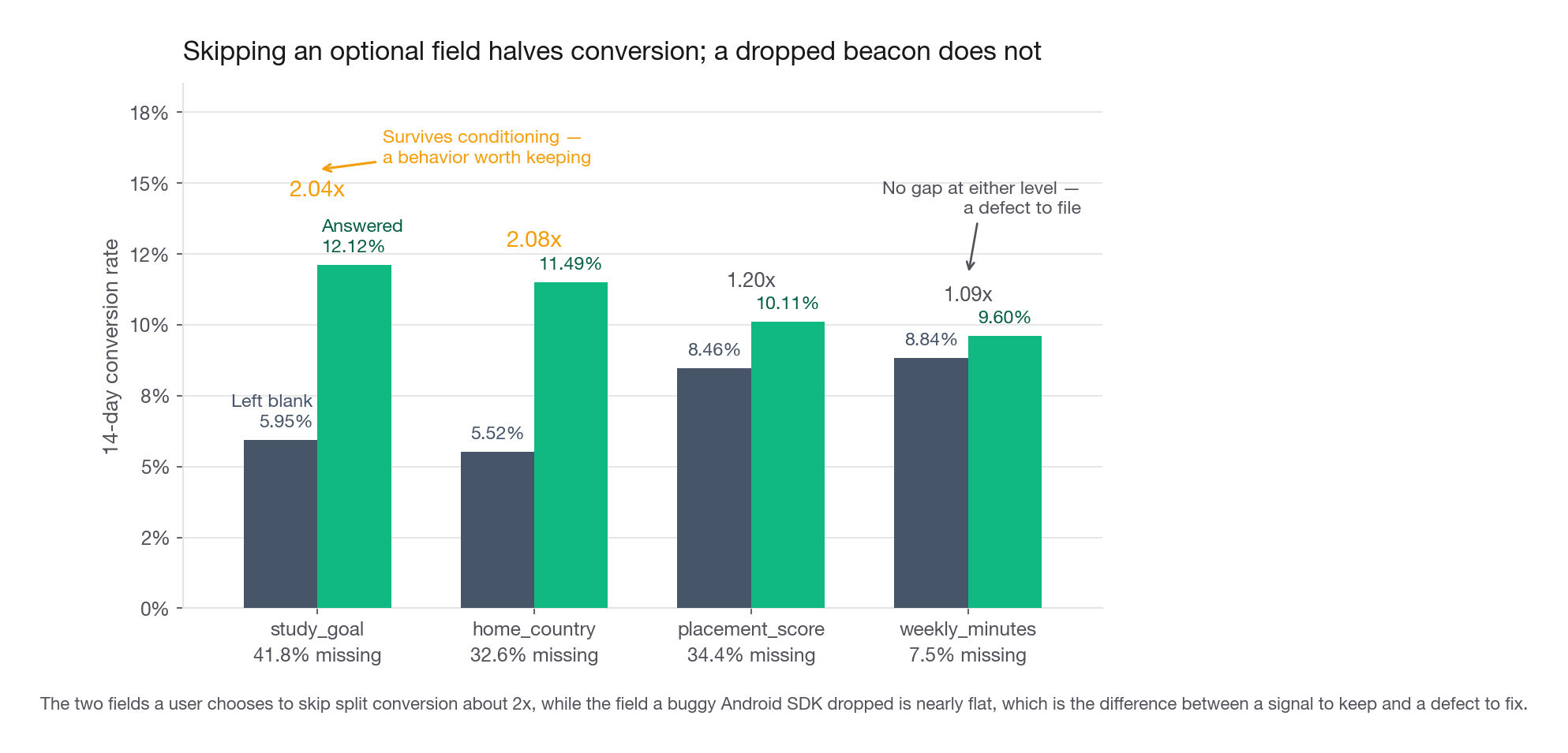
study_goal 41.8 5.95 12.12 2.04
home_country 32.6 5.52 11.49 2.08
placement_score 34.4 8.46 10.11 1.20
weekly_minutes 7.5 8.84 9.60 1.09Read that table the way an interviewer wants it read. Accounts that skipped the onboarding goal question convert at 5.95 percent; accounts that answered convert at 12.12 percent. The content of the answer is irrelevant, we never looked at whether they chose travel or work. The act of answering is worth a factor of two.
The fourth row barely moves at all, 8.84 against 9.60. That is the MAR column, and the honest reading is that the gap never rose above noise in the first place: a ratio of 1.09, and 1.4 standard errors away from no gap at all. Condition on device and watch what happens, which in this table is nothing:
by_dev = (mar.assign(miss=mar["weekly_minutes"].isna())
             .groupby(["device", "miss"])["converted"]
             .agg(n="size", conv="mean"))
by_dev["conv"] = (100 * by_dev["conv"]).round(2)
print(by_dev.to_string())
n conv
device miss
android False 16047 9.55
True 2782 8.81
ios False 13346 9.87
True 143 9.09
web False 7608 9.25
True 74 9.46Within Android, 8.81 against 9.55 on 2,782 missing rows. The standard error on that gap is about 0.59 percentage points, so it sits roughly 1.3 standard errors from zero, which is nothing.
Now say precisely what that shows, because this is the sentence candidates oversell. The gap did not collapse: 0.77 points marginally, 0.74 inside Android, 97 percent of what it started as. Conditioning removed nothing because there was nothing to remove. device is where the bug lives, but device barely moves conversion here, 9.44 percent on Android against 9.86 on iOS and 9.25 on web, a chi-squared p of 0.28. A column that does not separate the outcome cannot absorb a gap in it, so composition was never the explanation, and neither the 1.4 standard errors before nor the 1.3 after is distinguishable from zero. The flag carries no signal at either level.
That is a weaker claim than "it collapses", it is the true one, and it is the better reflex. The trap is the seductive story: you like the mechanism, the numbers point vaguely the right way, and you narrate a collapse the arithmetic never delivered. "How big was the gap before you conditioned, and was that one significant?" is the follow-up that catches it. Where the broken platform really does convert worse, a real marginal gap shrinks toward zero inside device, and collapse is the right word.
So state the rule the numbers support. Missingness whose gap is not distinguishable from zero, before or after you condition on the suspected cause, is a defect to fix. Missingness that survives conditioning is a behavior to keep. That distinction is the single most useful thing on this page.
There is one more feature hiding in this table, and it is free. Count how many optional fields each account left blank.
opt = ["study_goal", "home_country", "placement_score", "weekly_minutes"]
mar["n_blank"] = mar[opt].isna().sum(axis=1)
print(mar.groupby("n_blank")["converted"]
         .agg(n="size", conv=lambda s: round(100 * s.mean(), 2))
         .to_string())
n conv
n_blank
0 10569 14.55
1 15881 9.75
2 10202 5.94
3 3166 3.70
4 182 4.40A monotone ladder from 14.55 percent to 3.70 percent across the first four steps, with the last cell too small to read. Profile completeness is a legitimate engagement proxy costing one line of pandas and no new logging. It adds nothing on top of the individual indicators here, since they already encode it, but in a linear model or a shallow tree it is often the cleaner way to spend one degree of freedom.
Interview tip: Report the gap in the units the business uses. "Accounts that skip the goal question convert at 5.95 percent against 12.12 percent" lands. "The missingness indicator has a chi-squared p below 0.001" does not.
The missing-indicator pattern
Two steps, and this is the default you should reach for.
Step one: record that the value was absent. For a continuous column, add a binary companion feature. For a categorical column, add a new level rather than a separate binary, because the new level already is the binary.
Step two: put something in the hole that is harmless to your model family. The fill value is not an estimate of the truth. It is a placeholder chosen so the model can ignore it, because step one already carried the information. That is the part people miss, and it is why the "best" fill value depends entirely on the algorithm.
CATS = ["device", "channel", "study_goal", "home_country"]
NUMS = ["placement_score", "weekly_minutes"]

def encode(frame, medians, add_flags=True, flag_cols=NUMS):
    out = frame.copy()
    if add_flags:
        for c in flag_cols:
            out[f"{c}_is_missing"] = frame[c].isna().astype(int)
    for c in CATS:
        out[c] = out[c].fillna("__unknown__")
    for c in NUMS:
        out[c] = out[c].fillna(medians[c])
    return out

train = mar.sample(frac=0.7, random_state=7)
medians = {c: train[c].median() for c in NUMS}
print(encode(mar.head(3), medians)[["study_goal", "placement_score",
                                    "placement_score_is_missing"]].to_string())
Note that medians is computed on train only. That is not decoration, and the next section explains what it is protecting you from. Note also the default of flag_cols: in production this function flags the numerics and nothing else, because the categoricals already carry their own missingness in the __unknown__ level and a second copy of a column is not a feature.
Do you need both the unknown level and the flag?
That default is a claim, so measure it. Here is the ablation, a histogram gradient boosted classifier on a 70/30 split, scored by average precision on the holdout. Base rate on the holdout is 9.54 percent, so a random ranker scores 0.0954 and "lift" is the ratio. Read the two column headers as harness settings: "Explicit missing flags" means calling encode with flag_cols=CATS + NUMS, so every column with a hole gets its own binary, categoricals included, which is deliberately not the production default above; "No, mode-filled" swaps the __unknown__ level for the train-set mode, a path encode does not offer because the grid is about to show why you would not want it.
| Unknown level for categoricals | Explicit missing flags | PR-AUC | ROC-AUC | Lift over random |
|---|---|---|---|---|
| No, mode-filled | No | 0.1939 | 0.6834 | 2.03x |
| No, mode-filled | Yes | 0.2027 | 0.6919 | 2.12x |
| Yes | No | 0.2002 | 0.6931 | 2.10x |
| Yes | Yes | 0.2007 | 0.6942 | 2.10x |
Three things to take from that grid.
First, the row that erases missingness entirely, mode-filled with no flags, is worst on both metrics. It costs about 4.5 percent of PR-AUC relative, and the loss is pure: you had the information, deleted it, and got nothing back.
Second, you need one of the two mechanisms, not both. An __unknown__ level and a study_goal_is_missing flag are the same column written twice; adding the second moved PR-AUC by 0.0005, which is noise. Run permutation importance on the model with both and the categorical flags come out near zero. Candidates who see that conclude the indicators do not work. They do work, they are just already in there.
Third, quote that 4.5 percent honestly: it is real but modest. Marlow's weekly_minutes is a strong engagement proxy present 92.5 percent of the time, so the model still has good signal after you break the other columns. On a table where the informative columns are the optional ones, the gap is far larger. Sell the reasoning, not the technique.
Sentinel fill and why it is model-specific
For tree-based models, an alternative to the flag is to fill the hole with a value far outside the observed range, say negative 999 for a score that runs 0 to 100. A tree only ever asks "is this feature above or below a threshold", so it will happily learn a split at negative 500 that isolates exactly the missing group. The sentinel becomes the indicator.
Do the same in a logistic regression and you have poisoned the model. The coefficient is a slope applied to the raw value, so a row at negative 999 drags the entire fitted relationship toward itself. An L2 penalty does not save you: the problem is the design matrix, not the variance of the estimate.
| Model family | Categorical fill | Continuous fill | Add explicit flag | Sentinel like -999 |
|---|---|---|---|---|
| Logistic regression | New unknown level | Median, computed on train | Required | Never, it wrecks the slope |
| Random forest, plain GBM | New unknown level | Median or sentinel | Optional if you use a sentinel | Safe |
| HistGradientBoosting, LightGBM, XGBoost | New unknown level | Leave the NaN in place | Redundant, the split rule handles it | Unnecessary |
| k-nearest neighbours | New unknown level | Median, and scale afterwards | Required | Never, it dominates the distance |
| Naive Bayes | New unknown level | Median | Required | Never, it breaks the likelihood |
The third row is what you will actually use, so know the mechanism. Histogram-based boosters handle NaN natively: at each split the algorithm sends all missing rows left, then all missing rows right, scores both, and keeps the better option. It is learning the indicator inside the split rule, so an explicit flag adds nothing the model does not already have. Very few candidates can say that when asked what the library does with NaN.
Do not reach back to the ablation grid for evidence, though. Every row of that grid fills all four columns before fitting, so the design matrix that reached the model held zero holes and the native path was never exercised there. It cannot be why row four gains 0.0005 over row three; that gain is small for the mundane reason two paragraphs above, the flag and the level being the same column twice. "Did your ablation leave the NaNs in?" is a fair follow-up, and for that grid the answer is no.
The native path needs its own run: leave the numeric and categorical holes as NaN and let the booster route them.
| Configuration | Holdout PR-AUC | Holdout ROC-AUC |
|---|---|---|
| Native NaN, no explicit flags | 0.2008 | 0.6938 |
| Native NaN plus flags on all six columns | 0.2008 | 0.6938 |
Identical to four decimals at this seed, which is luckier than you should expect; across seven model seeds the two average 0.2009 and 0.2011. Quote the seed average, not the coincidence. That is the evidence behind "redundant" in the third row of the model-family table above.
Interview tip: If you name a fill value, name the model family in the same breath. "Median plus an indicator, because we are fitting a logistic regression" is a complete answer; "median" on its own invites the follow-up you will fumble.
Imputation: which option, and when it is safe
Three of those rows deserve the numbers behind them.
Complete-case analysis lies about its own accuracy
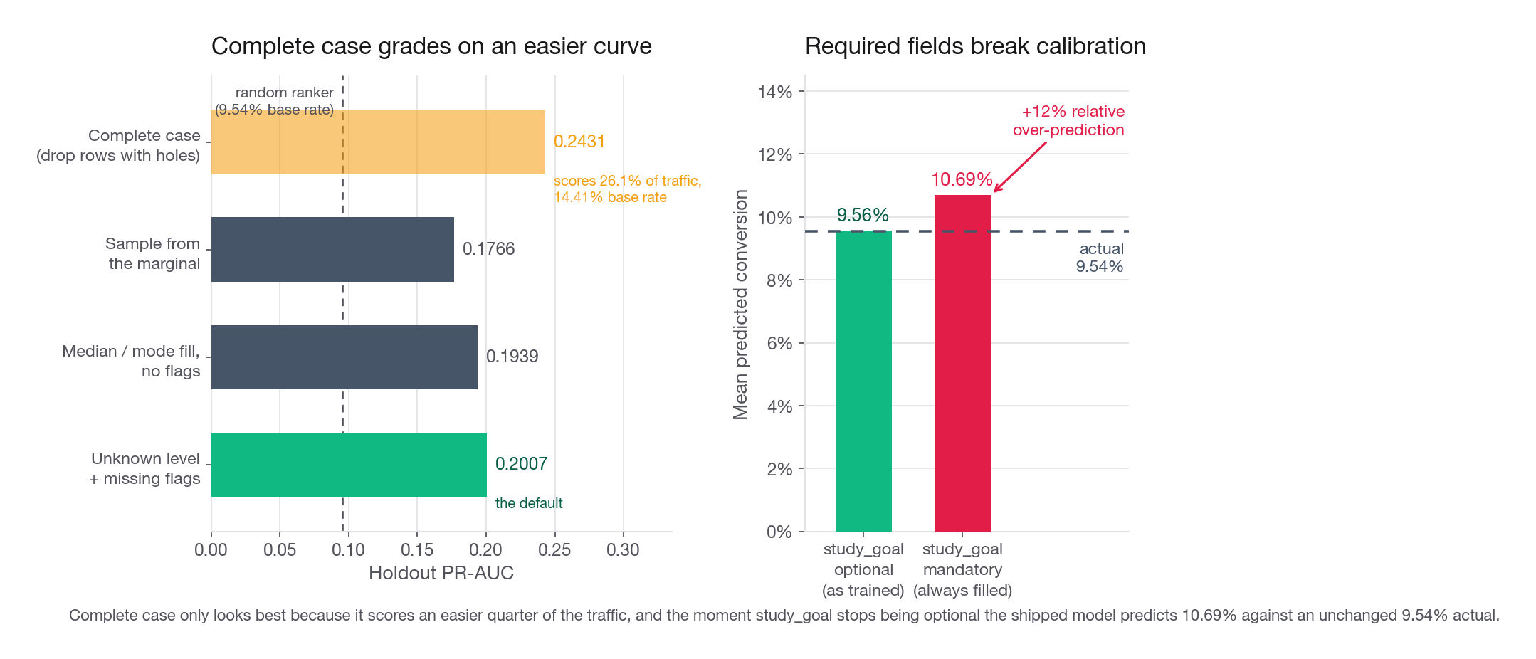
Drop every Marlow row with any hole and you keep 26.1 percent of the table. Train and evaluate on that subset and the model scores PR-AUC 0.2431, comfortably above the 0.2007 you get from the indicator approach on the full table. A candidate who stops there reports the wrong winner.
Two problems. First, PR-AUC is not comparable across populations with different base rates. The complete-case holdout has a base rate of 14.41 percent, because complete profiles convert better, against 9.54 percent on the full holdout. Normalize and the ordering flips: 0.2431 over 0.1441 is 1.69x lift, while 0.2007 over 0.0954 is 2.10x. The complete-case model is not better, it is grading on an easier curve.
Second, and fatal on its own, that model can only score 26.1 percent of arriving traffic. The other 73.9 percent shows up with a hole and the pipeline has no defined behavior, so someone adds a fallback rule at 3am and you now have an unmeasured second model serving three quarters of your users.
Interview tip: When you compare models trained on different subsets, state the base rate of each evaluation set before you state the score. PR-AUC scales with prevalence, and comparing raw values across populations is the most common quiet mistake in an unbalanced-class answer.
Sampling from the marginal is the worst of the reasonable options
There is an argument that sounds principled: fill each hole by drawing at random from that column's observed values, so the column's distribution is unchanged. Frequent levels get filled often, rare levels rarely, and no artificial spike appears at the median.
It scores worst of the four strategies tested here, PR-AUC 0.1766 against 0.2007, and it does two damaging things at once. It scatters the missing group across every level, so no split can isolate them and the flag is gone. And on an MNAR column it preserves a distribution that was never the population distribution: test takers average 58.8, the population averages 52.9, so every imputed row reproduces the selection bias faithfully.
Model-based imputation: rarely the answer in an interview
Iterative imputation, where each column with holes is regressed on the others in rounds, and kNN imputation, where holes are filled from similar rows, both do real work when a column is MAR and genuinely correlated with columns you have. Say two things if you propose one. That you would still add the indicator, because a predicted value and an observed value are not the same evidence and the model deserves to know which it is holding. And that you would fit the imputer on training rows only and freeze it, because a kNN imputer borrowing neighbours across the train/test boundary is a leak with extra steps.
Leakage: three flavors, and only one of them is big
Candidates recite "fit the imputer on train only" without knowing what it protects against or what it is worth. Here are all three flavors, measured.
Flavor one: the fill statistic sees the holdout
You compute the median of placement_score over the whole frame, then split. The holdout rows contributed to a number that was used to build features for the holdout.
Measured on Marlow: honest PR-AUC 0.2002, leaked 0.1983. The leak is worth less than nothing here, which is the honest result and you should say so.
That does not make the discipline optional, and here is the argument that holds. A median over 28,000 rows and a median over 40,000 differ in the third decimal place, so at this size the leak is invisible; shrink to 600 rows and it is still invisible, because a median is robust by construction. The leak becomes real when the statistic is fragile: a per-group median where some groups have four rows, a target-encoded category mean, a kNN imputer whose neighbours are individual holdout rows. Fitting on train only is insurance you pay for once, in a pipeline definition, and it is the only way to get an offline number you can reproduce.
Flavor two: the imputer sees the label
This one is not subtle, and it is the one that actually appears in real notebooks, usually because somebody wanted a "smarter" fill.
# WRONG. Never do this. Shown so you can recognise it in a review.
by_label = mar.groupby("converted")["placement_score"].median()
leaked = mar["placement_score"].fillna(mar["converted"].map(by_label))
Fill each missing score with the median score of accounts that share its outcome, and the holdout PR-AUC goes from 0.2002 to 0.5878, ROC-AUC from 0.6931 to 0.8754. Nearly a 3x improvement in average precision, from a feature that cannot exist at serving time, because at serving time the label is what you are trying to predict.
The tell is always the same: the imputation recipe references the target, directly or through a group key derived from it. Any post-outcome field counts, so filling a missing plan_tier with the tier the account eventually bought is the same bug in a different hat.
Flavor three: recomputing the statistic at serving time
This is the one the textbooks skip and production punishes. You wrote a scoring job that reads a batch, computes the median of each numeric column over that batch, fills, and predicts. It works in the notebook, where the batch is a nicely balanced test set.
Then marketing runs a push that swings the mix, Android share goes from 46.9 percent to 75 percent, and your fill values move under you. In Marlow the medians barely budge, 58.8 to 58.2 and 44.8 to 44.5, and the scores are indistinguishable, so I will not pretend this is an accuracy emergency here. The real failure is structural. A real-time endpoint receives one row; there is no batch to take a median over. The online code path therefore cannot be the offline one, someone writes a second implementation, and the two drift with nobody watching. Freezing the fill values into the artifact makes one path serve both.
The fix for all three is the same object, and it is worth being able to write from memory:
from sklearn.compose import ColumnTransformer
from sklearn.pipeline import Pipeline
from sklearn.impute import SimpleImputer
from sklearn.preprocessing import OneHotEncoder, StandardScaler
from sklearn.linear_model import LogisticRegression

num = Pipeline([("fill", SimpleImputer(strategy="median", add_indicator=True)),
                ("scale", StandardScaler())])
cat = Pipeline([("fill", SimpleImputer(strategy="constant", fill_value="__unknown__")),
                ("oh", OneHotEncoder(handle_unknown="ignore"))])

pipe = Pipeline([
    ("prep", ColumnTransformer([("n", num, NUMS), ("c", cat, CATS)])),
    ("clf", LogisticRegression(max_iter=2000)),
])
add_indicator=True is the missing-indicator pattern in one keyword, and handle_unknown="ignore" stops an unseen category at serving time from raising. Because the whole thing is one estimator, pipe.fit(X_train, y_train) learns the medians from training rows only and pipe.predict_proba(X_new) reuses those frozen numbers for a batch of a million rows or a batch of one.
Notice what is absent from that block: no class_weight="balanced". At a 9.54 percent base rate on 28,000 training rows the fit needs no rescuing, and reweighting buys almost nothing on ranking, PR-AUC 0.2024 against 0.2022, while wrecking the probability scale: mean predicted conversion 45.07 percent against an actual 9.54 percent, a 4.7x over-prediction. Unweighted, the same pipeline predicts 9.55 against 9.54. Reach for class weights when the fit is collapsing to a constant, not by reflex, because the calibration monitor in the checklist below is meaningless on a model whose probabilities were thrown away before it shipped.
Interview tip: If an interviewer asks how you avoid imputation leakage, answer with the artifact rather than the rule. "The imputer is a fitted step inside the pipeline, so the fill values ship with the model" ends the question; "I fit on train only" invites three more.
The product read: missingness is a behavior log
You have established that Marlow accounts skipping the goal question convert at half the rate, so the modeling half of the answer is done. Almost every candidate stops there, and the interviewer is waiting for the other half, because this is a product loop.
Reframe the finding in the product manager's language: 41.8 percent of new accounts decline the first optional question we ask, and that group is worth half as much. That is not a data quality ticket, it is a funnel finding about onboarding.
Four things a team can do with it, in increasing order of ambition:
Score with it. Feed the indicator into whatever ranks accounts for lifecycle email, trial extensions, or a sales touch. It is free and available at minute zero, before any usage history exists, which is exactly when cold-start models are starving.
Trigger on it. An account that skipped the placement test gets a different day-two message than one that finished it. Missingness is one of the cheapest segmentation variables you will ever find.
Change what you ask. A question skipped 41.8 percent of the time is placed badly, phrased badly, or asked too early. That is a design experiment with a clear metric.
Change whether you ask. Making the field mandatory is tempting and usually wrong. Read on.
The causal trap, and the model-rot trap behind it
The tempting recommendation is: skipping predicts churn, so stop letting people skip. Two problems, and naming both is what separates a senior answer.
The causal problem is obvious. Skipping does not cause low intent; low intent causes skipping. Forcing a disengaged user through one more mandatory screen converts nobody and adds friction for the users who would have converted anyway. If a team insists, the honest design is an onboarding experiment with signup-to-activation as the primary metric and a completion-rate guardrail, not a rollout justified by this correlation.
The second problem is the one candidates never raise, and it is the strongest thing you can say here. Making the field required destroys the feature. Simulate it: take the trained model, then feed it a future population where study_goal is always populated because the team made it mandatory.
| Population | PR-AUC | ROC-AUC | Mean predicted conversion | Actual conversion |
|---|---|---|---|---|
| Holdout as trained | 0.2007 | 0.6942 | 9.56 percent | 9.54 percent |
| After the field becomes required | 0.1940 | 0.6828 | 10.69 percent | 9.54 percent |
Ranking degrades modestly, about 3.3 percent of PR-AUC. The calibration damage is worse and far more visible to the business: mean predicted conversion jumps to 10.69 percent while true conversion has not moved. Every account now looks like a complete-profile account, so the model over-predicts by roughly 12 percent relative, silently, until someone notices the forecast running hot.
This is the general hazard with behavioral features drawn from product surfaces: a product change can rewrite your feature's meaning without touching a line of your code. A logging migration, a redesigned onboarding flow, a privacy setting that starts defaulting to off, each moves a missingness rate. So when you ship a model leaning on missing-indicators, ship a monitor on the missingness rate of every one of those columns, alerting on a week-over-week shift beyond a few points. That sentence is often the most senior thing said in an entire modeling interview.
What the interviewer asks next
Four follow-ups that arrive in almost every version of this conversation, compressed to what you would actually say.
"Is the indicator just a proxy for engagement?" Often yes, and that is fine, because it exists at minute zero when no engagement history does. Once you have two weeks of usage it usually shrinks in importance. It earns its place in cold start; check whether it still earns it at day thirty.
"What if the missingness is caused by a bug you have not found?" Then you are training the model to predict who is on the broken client, which holds until the fix ships and then collapses. The tell is concentration: holes clustered in one platform, one app version, or one date range are a defect. The Android beacon column here is exactly that shape, so I would drop its flag and file a ticket rather than model it.
"A column is 97 percent missing. Drop it?" Not on the percentage alone. Check the target rate on the 3 percent present. If it splits the outcome sharply, keep the indicator and drop the values: the fact that a rare thing happened is usable even when the value is too sparse to estimate from.
"How would you handle a missing target rather than a missing feature?" Completely differently, and say so out loud, because it is a common trap. A missing label is a selection or semi-supervised problem, not an imputation one. Impute a label and you train the model on its own guesses. If labels are missing non-randomly, for example because only some accounts were ever reviewed, you need inverse-probability weighting or an explicit selection model.
Common traps
Treating the percentage missing as the whole diagnosis. Two columns at 34 percent missing can need opposite treatments. The fix is the split-by-target audit plus the write path question, together under a minute.
Median-filling an MNAR column with no indicator. The most expensive default in the topic. Here it assigns 58.7 to a group whose true median is near 41.5, in the same direction for every affected row. The fix is an indicator, native NaN handling, or a sentinel on a tree model.
Sampling from the observed distribution because it "preserves the distribution". It preserves the distribution of the people who answered, which on a self-selected column is the wrong one, and it scatters the missing group so no split can find them. Worst of every strategy tested here.
Reporting complete-case accuracy without reporting coverage. PR-AUC 0.2431 on 26.1 percent of traffic does not beat 0.2007 on all of it, and after normalizing by base rate it does not beat it on the metric either.
Letting the label into the imputation. Group medians keyed on the outcome, fills from a post-outcome column, target encoding fit on all rows. The holdout number gets beautiful and production stays flat. Grep imputation code for the target's name.
Recomputing fill values on the scoring batch. Impossible for single-row serving, so it forces a second implementation of your preprocessing and the two drift. Freeze the statistics into the fitted pipeline.
Recommending the optional field be made mandatory. Confuses correlation with causation and silently breaks the feature: predicted conversion inflates about 12 percent relative the moment the field is always populated.
Shipping missing-indicators with no monitoring. Product teams change onboarding without telling the modeling team. A weekly missingness-rate alert per column costs an hour and catches it.
Reciting the three mechanisms as if the data could tell you which applies. It cannot separate the last two. Say so, then say how you would find out.
Quick self-check
Answer these out loud, in full sentences, the way you would in the room.
A column is 34 percent missing and the outcome rate is identical for the missing and present groups. Give two different reasons that could be true, and say what you would do differently in each case.
Your interviewer says "just median-impute it". Give the one-sentence rebuttal, then the follow-up question you would ask before agreeing or disagreeing.
You add a missing-indicator for a categorical column that you have already given an
unknownlevel. What do you expect the indicator's importance to be, and why?Explain, without using the word leakage, why the imputation medians must come from the training rows only, and give one case where it changes the answer materially and one where it does not.
Your model uses six missing-indicators. The onboarding team is about to make three of those fields mandatory. Say what breaks first, ranking or calibration, and what you would put in place before the change ships.
"We run a survey where unhappy customers tend not to respond. How would you estimate true average satisfaction?" Name the mechanism, say why the observed mean is biased in a known direction, and give one approach that beats the observed mean.
If question 3 or 5 gave you trouble, reread the ablation grid and the model-rot table. Those two separate candidates who have read about missing data from candidates who have shipped a model that depended on it.