4.3 Randomization and Its Failure Modes
Find the core decision, design, or behavior signal.
Turn the lesson into a concise response blueprint.
Name the trap you would avoid in a real interview.
Use these checkpoints as your reading path before diving into the full lesson.
- 1Why this matters in interviews
- 2How assignment actually works
- 3What the assignment service has to guar...
- 4A bucketer you can write on a whiteboard
- 5Assignment mechanisms compared
An experiment readout is a claim about one difference between two groups of people. Every failure mode in this lesson is a way that claim quietly becomes false while the dashboard keeps rendering a confident number to three decimals. The decision here is narrow and comes before any statistics: given a finished experiment, do you trust the assignment enough to read the metric at all, and if not, which repair is legitimate. By the end you should be able to run the four pre-readout checks in order, name what each can and cannot catch, and say what you do when one fails.
Why this matters in interviews
The previous two lessons handed you a design and a sample size. This one separates candidates who can describe an experiment from candidates who have shipped one.
Interviewers probe this because the failure is invisible. A broken power calculation announces itself with an embarrassingly wide interval. A broken assignment gives a tight interval around the wrong number, and nothing on the results page looks off. The only defense is a habit, and the interviewer wants to know whether you have it.
The moment it gets scored is predictable. You present a result, the interviewer says "treatment is up four percent, would you ship it", and waits. A weak candidate answers the question asked. A strong candidate first asks for arm counts against the intended split, covariate balance, exposure rate in both arms, and the pre-period. Every one of those four has killed a real launch.
Here is the difference in one exchange.
Weak: "Lift is 4.1 percent at p below 0.01, so ship it and monitor the guardrails."
Stronger: "Before the lift, three numbers. The arms are 239,670 and 233,722 against a designed even split, a 1.3 percent shortfall in treatment that cannot be chance at this sample size, so something is dropping treatment rows and whatever drops rows is probably not dropping them at random. Second, exposure is 44 percent in both arms, a dilution question, and the interval on that gap is too wide to call it clean. Third, I want the pre-period A/A. My recommendation is do not ship, and the reason is a logging bug, not a statistics problem."
The second answer takes forty seconds and carries the whole signal.
Interview tip: Rehearse one sentence you say before every readout: "counts, balance, exposure, pre-period, then the metric." Saying it unprompted beats any test statistic you can name.
How assignment actually works
Most candidates describe randomization as a coin flip per user. No production system works that way, and the ways real systems do work are where the bugs live. If you cannot describe the mechanism you cannot debug it.
What the assignment service has to guarantee
Four properties, each of which fails somewhere in the wild.
Deterministic. The same unit lands in the same arm on every request, on every server, after every deploy. A per-request coin flip gives a user a different experience on each page load, which is not an experiment, it is noise generation.
Uniform. Every bucket gets the same expected share. A hash with poor avalanche behavior, or a modulo taken on an identifier with structure in its low digits, produces buckets of unequal size.
Independent across experiments. Otherwise a unit in treatment for the banner test is also in treatment for the checkout test and you cannot separate the effects.
Stateless. The arm comes from the identifier alone. A stored assignment table works until the write fails or the cache expires, and then units silently flip arms mid-run. Hashing is the mechanism that satisfies all four.
A bucketer you can write on a whiteboard
Concatenate an experiment-specific salt with the identifier, hash it, reduce the digest to an integer, take that modulo the bucket count, and map bucket ranges to arms.
import hashlib

def bucket_of(unit_id, salt, buckets=1000):
    key = f"{salt}|{unit_id}".encode()
    digest = hashlib.blake2b(key, digest_size=8).digest()
    return int.from_bytes(digest, "big") % buckets

def arm_of(unit_id, salt, control_width=500, buckets=1000):
    return "control" if bucket_of(unit_id, salt, buckets) < control_width else "treatment"
Three details there are load-bearing. The salt sits inside the hashed key rather than being appended after, which is what makes two experiments independent. The hash is a real digest, not Python's built-in hash, which is randomized per process for strings, so a restart reassigns everybody. And there are a thousand buckets, not two: buckets are the unit of traffic allocation, so ramping from 5 to 50 percent widens a bucket range while every unit keeps its bucket.
Run it on 200,000 synthetic identifiers and all four properties are visible at once.
import numpy as np
from scipy import stats

ids = [f"lv_{i}" for i in range(200_000)]
banner = np.array([arm_of(i, "listing_banner_2026_09") == "treatment" for i in ids])
checkout = np.array([arm_of(i, "checkout_copy_2026_09") == "treatment" for i in ids])
banner_again = np.array([arm_of(i, "listing_banner_2026_09") == "treatment" for i in ids])

counts = np.bincount([bucket_of(i, "listing_banner_2026_09") for i in ids], minlength=1000)
print(round(banner.mean(), 4), round((banner == checkout).mean(), 4),
      round((banner == banner_again).mean(), 4),
      round(stats.chisquare(counts).pvalue, 3))
0.4983 0.4986 1.0 0.864The banner test splits 49.83 percent into treatment. Agreement with the checkout test is 49.86 percent, which is chance, so the two are independent. Agreement with itself is exactly 1.0, so it is deterministic. The thousand bucket counts pass a uniformity test at p equal to 0.864.
Now reuse listing_banner_2026_09 as the salt for the checkout test. Agreement jumps to 1.0, the treatments are perfectly confounded, and neither result means anything. This is the most common bug at a company that just built its own platform, because a constant salt looks harmless until two tests overlap.
Interview tip: Asked to design an assignment service, say "hash of salt plus id, modulo a thousand buckets, arms are bucket ranges" in one breath, then explain why the salt sits inside the hash. That sentence signals you have seen a real platform.
Assignment mechanisms compared
The second row earns a concrete failure. Suppose identifiers are a millisecond timestamp times a thousand plus a per-datacenter counter, east using 0 through 499 and west using 500 through 999. Then id % 1000 puts every east request in control and every west request in treatment, and the experiment is a comparison of two datacenters serving different latency to different populations. The split ratio looks like a perfect fifty-fifty throughout.
A dataset to work on
The running example is Loomlane, a marketplace for handmade textiles. The experiment adds a promoted-listing banner to category pages and the primary metric is the share of assigned visitors who order within seven days. This block builds the assignment log deterministically, and everything downstream assumes the dataframe loom exists.
import numpy as np
import pandas as pd

SEED = 4703
rng = np.random.default_rng(SEED)

N = 480_000
device = rng.choice(["ios", "android", "web"], N, p=[0.31, 0.44, 0.25])
tier = rng.choice(["low", "mid", "high"], N, p=[0.27, 0.45, 0.28])
country = rng.choice(["US", "CA", "GB", "AU"], N, p=[0.52, 0.14, 0.22, 0.12])
channel = rng.choice(["organic", "paid", "email"], N, p=[0.47, 0.34, 0.19])
logged_in = rng.random(N) < np.where(device == "web", 0.38, 0.71)
prior_orders = rng.poisson(np.where(logged_in, 2.1, 0.3))

bucket = rng.integers(0, 1000, N)
arm = np.where(bucket < 500, "control", "treatment")

drag = np.select([tier == "low", tier == "mid"], [0.021, 0.006], 0.0)
p_reach = 0.34 + 0.18 * logged_in + 0.06 * (channel == "email") - 0.10 * (tier == "low")
reached = rng.random(N) < p_reach

p_order = (0.052 + 0.026 * logged_in + 0.004 * np.minimum(prior_orders, 6) - drag
           + 0.011 * ((arm == "treatment") & reached))
ordered = rng.random(N) < p_order

lost = (arm == "treatment") & (rng.random(N) < np.where(tier == "low", 0.09, 0.004))

loom = pd.DataFrame({
    "visitor_id": np.arange(1, N + 1), "arm": arm, "bucket": bucket,
    "device": device, "device_tier": tier, "country": country, "channel": channel,
    "logged_in": logged_in.astype(int), "prior_orders": prior_orders,
    "reached_listing": reached.astype(int), "ordered": ordered.astype(int),
})
loom = loom.loc[~lost].reset_index(drop=True)
print(loom.shape, loom["arm"].value_counts().to_dict())
(473392, 11) {'control': 239670, 'treatment': 233722}The planted bug is the lost line: the treatment build loses 9 percent of low-tier sessions before they reach the assignment log, and 0.4 percent of everything else. In the real version you have the dataframe and a deadline, not the generator. The true effect built into this data is 0.481 percentage points on the assigned population, a 7.4 percent relative improvement. That comes off the generator, not the sample: the banner adds 0.011 to the order probability, but only for treatment visitors who reach a category page, and 43.7 percent do, so 0.011 times 0.437 is 0.0048. Hold it.
Check one: sample ratio mismatch
Sample ratio mismatch, usually shortened to SRM, is the gap between the split you designed and the split you observe in the logs. It is first because it is cheapest, most sensitive, and the only check that flags a whole category of bugs balance testing cannot see.
The check
from scipy import stats

n = loom.groupby("arm").size()
total = int(n.sum())
expected = [total / 2, total / 2]
chi2, p = stats.chisquare([n["control"], n["treatment"]], expected)
print(n.to_dict(), round(n["treatment"] / total, 5), round(chi2, 1), f"{p:.2e}")
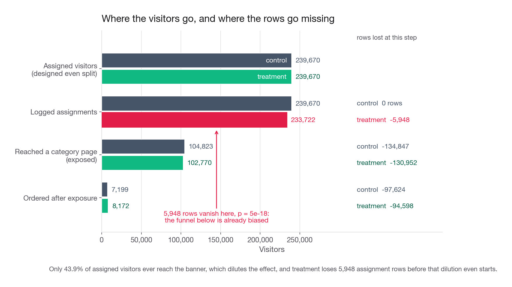
{'control': 239670, 'treatment': 233722} 0.49372 74.7 5.38e-18Treatment holds 49.372 percent of logged assignments instead of 50, a shortfall of 2,974 rows against an expectation of 236,696, which is 1.24 percent light.
Convert that shortfall into a loss rate before you quote it. A mechanism deleting a fraction f of one arm's rows leaves that arm an observed share of (1 - f) / (2 - f), so a relative shortfall s implies f = 2s / (1 + s), roughly twice the shortfall, because the deleted rows leave the denominator as well as the numerator. Here 1.24 percent light means about 2.5 percent of treatment's rows never reached the log.
Two reactions are both wrong: shrugging because 1.24 percent is small, and "fixing" it by subsampling control to 233,722 rows. Neither engages with the fact that a mechanism is deleting treatment rows, and it gets to choose which ones.
Why the threshold is 0.001 and not 0.05
You run this test on every experiment, so at 0.05 you would false-alarm on one in twenty and the team would learn to ignore the alert within a month. The convention is p below 0.001, sometimes 0.0001 at very large platforms, and it is still brutally sensitive because the test has your entire sample behind it.
| Observed treatment share | 20,000 rows | 100,000 rows | 473,392 rows | 2,000,000 rows |
|---|---|---|---|---|
| 49.9 percent | 0.78 | 0.53 | 0.17 | 0.005 |
| 49.7 percent | 0.40 | 0.058 | 0.000037 | 2e-17 |
| 49.4 percent | 0.090 | 0.00015 | 1.5e-16 | 1e-64 |
| 49.0 percent | 0.0047 | 2.5e-10 | 4.4e-43 | 5e-176 |
Read the third column: at this size a six-tenths-of-a-point shortfall is a one-in-a-quadrillion event under a fair split. The smallest shortfall catchable at p below 0.001 is 2.3 percent at 20,000 rows, 1.0 percent at 100,000, 0.48 percent at 473,392, and 0.23 percent at two million. Bigger experiments detect smaller bugs, not only smaller effects.
Interview tip: Quote an SRM as a row deficit and a p-value, never a percentage alone. "Treatment is short 2,974 rows, p is 5e-18" ends the argument; "treatment is down about a percent" invites someone to call it noise.
Localize before you theorize
An overall SRM says something is broken. Splitting it by every logged dimension says what.
rows = []
for value, g in loom.groupby("device_tier"):
    c, t = int((g.arm == "control").sum()), int((g.arm == "treatment").sum())
    chi2, p = stats.chisquare([c, t], [(c + t) / 2] * 2)
    rows.append({"segment": value, "control": c, "treatment": t,
                 "share_t": round(t / (c + t), 4), "p": f"{p:.1e}"})
print(pd.DataFrame(rows).to_string(index=False))
segment control treatment share_t p
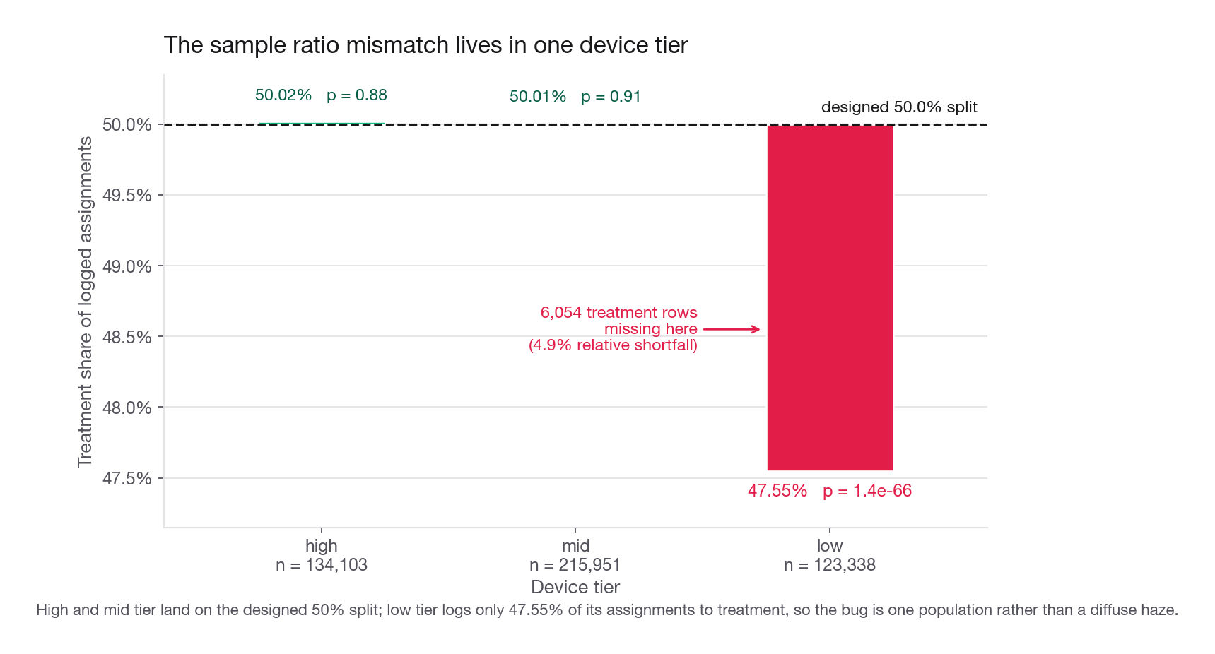
high 67025 67078 0.5002 8.8e-01
low 64696 58642 0.4755 1.4e-66
mid 107949 108002 0.5001 9.1e-01High and mid tier sit exactly on the line. Low tier is at 47.55 percent, a 4.9 percent relative shortfall. Run it through the conversion: 2 * 0.049 / 1.049 is 0.094, so about 9 percent of treatment's low-tier rows are gone. The bug is one population, not a diffuse haze, and that is what you take to the engineer: not "randomization looks off", but "treatment loses about 9 percent of low-tier sessions, roughly one in eleven, before the assignment beacon fires, and the other tiers are clean." Saying one in twenty would halve the bug in the engineer's head, and the engineer sizes the investigation off your number.
Run the same loop over country, channel, app version, and hour of day. App version and device tier are usually where it lands, because the mechanism is nearly always client-side: a slower render path, an extra redirect, a beacon firing after a screen transition instead of before.
The causes worth memorizing
| Symptom | Likely cause | How to confirm |
|---|---|---|
| Shortfall concentrated on one app version | Treatment build crashes or times out before the assignment event is sent | Crash rate by version and arm |
| Shortfall on slow devices or slow networks | Extra redirect or extra render in treatment, impatient sessions abandon first | Time from request to assignment event, by arm |
| Excess in treatment rather than a shortfall | Treatment fires the exposure event twice, or the dedupe key differs by arm | Distinct units versus event rows, by arm |
| Ratio off by a clean factor such as 2 to 1 | Configuration mismatch between the tool and the code | Read the config, not the data |
That last row matters more than it looks: many reported mismatches are someone changing the traffic allocation mid-run while the analysis still compares against the original design. Check the change log before you file a ticket.
When it is a real bug the default is: stop, find the mechanism, fix it, rerun. A bug that deletes rows non-randomly biases the estimate by an amount you cannot bound from the data you still have. Repairing the sample instead assumes the lost rows are missing at random given covariates you can see, and that is untestable, because the evidence that would test it is what went missing.
Check two: covariate balance
SRM asks whether the arms are the same size. Balance asks whether they hold the same kind of people. They often fail together and sometimes fail separately, so run both.
Variable by variable
for col in ["device_tier", "device", "country", "channel", "logged_in"]:
    table = pd.crosstab(loom[col], loom["arm"])
    chi2, p, _, _ = stats.chi2_contingency(table)
    print(f"{col:12s} chi2={chi2:7.1f}  p={p:.2e}")
device_tier chi2= 222.5 p=4.86e-49
device chi2= 4.1 p=1.26e-01
country chi2= 4.1 p=2.46e-01
channel chi2= 1.5 p=4.70e-01
logged_in chi2= 0.0 p=9.29e-01One variable is wrong and four are clean, which is the signature you want, because it points at a mechanism rather than at global chaos. Low tier is 26.99 percent of control and 25.09 percent of treatment.
Why the standardized difference alone would have missed this
Many teams clear balance with a standardized mean difference and a rule that anything under 0.1 is fine. For the low-tier indicator here that statistic is 0.043, comfortably inside the rule, and the rule would have been wrong. Effect-size thresholds were built for observational studies where you expect real imbalance and want to know if it is big enough to matter. In a randomized experiment the correct prior is that imbalance is exactly zero, so the question is not "is it large" but "is it larger than sampling noise allows", and at 473,392 rows sampling noise allows almost nothing.
Let a model do the searching
Checking twelve variables by hand misses interactions: the arms can match on device and on country while mismatching on Android-in-Canada. The general version turns balance into a supervised problem. Drop the outcome, make the arm the label, predict it from the covariates. If assignment worked, the arm is unpredictable by construction and no model beats a coin.
from sklearn.tree import DecisionTreeClassifier, export_text
from sklearn.ensemble import HistGradientBoostingClassifier
from sklearn.model_selection import cross_val_score

X = pd.get_dummies(loom.drop(columns=["visitor_id", "bucket", "arm",
                                      "ordered", "reached_listing"]))
y = (loom["arm"] == "treatment").astype(int)

tree = DecisionTreeClassifier(max_depth=3, min_impurity_decrease=2e-4,
                              class_weight="balanced", random_state=0)
tree.fit(X, y)
print(export_text(tree, feature_names=list(X.columns)))
print(cross_val_score(HistGradientBoostingClassifier(max_iter=120, random_state=0),
                      X, y, cv=4, scoring="roc_auc").mean().round(4))
|--- device_tier_low <= 0.50
| |--- class: 1
|--- device_tier_low > 0.50
| |--- class: 0
0.5093The tree, given fifteen candidate features and three levels of depth, makes exactly one split and it lands on the planted bug. That is what makes a tree the right first model here: it hands you the name of the broken variable instead of an importance ranking you then have to interpret.
The boosted model reaches an area under the curve of 0.5093. Drop the tier columns and it falls to 0.4997, which is chance. An AUC of 0.509 sounds like nothing and a junior reading calls it a useless model. It is not a model, it is a detector, and the finding is that the arms are distinguishable at all, which under a working assignment they should not be.
Three settings matter. Keep every level of every categorical when you dummy encode, because dropping a reference level can drop the broken one. Balance the class weights so the output reads as a split rather than a majority-class shrug. Set a minimum impurity decrease, or the default grows hundreds of noise splits and buries the finding.
Interview tip: Frame the adversarial classifier as "I train a model to guess the arm, and I want it to fail", then add "an AUC of 0.51 on half a million rows is a bug, not a weak model". That reframing is the whole answer.
Reweighting: what it buys and what it does not
Suppose engineering confirms the beacon loss is indiscriminate within low-tier sessions. Then you can poststratify: estimate the effect inside each tier and recombine using the pooled tier shares.
cell = loom.groupby(["device_tier", "arm"])["ordered"].mean().unstack()
weights = loom.groupby("device_tier").size() / len(loom)
diff = cell["treatment"] - cell["control"]
naive = loom.loc[loom.arm == "treatment", "ordered"].mean() - \
        loom.loc[loom.arm == "control", "ordered"].mean()
print(diff.round(5).to_dict(), round(float((diff * weights).sum()), 5), round(naive, 5))
{'high': 0.00549, 'low': 0.00517, 'mid': 0.00395} 0.0047 0.00503The naive difference is 0.503 percentage points, the poststratified estimate is 0.470, and the truth planted in the generator is 0.481. The naive estimate sits 0.022 points above the truth and the poststratified estimate 0.011 points below it, against a standard error of 0.073 points, since the t-test in check four returns t equal to 6.87 on that difference. One experiment cannot separate a 0.02-point bias from a standard error three times its size, and neither can you.
Repetition settles it. Regenerate this experiment 900 times: the naive estimator averages 0.512 points against a truth of 0.481, a 6.5 percent overstatement that never averages away, while the poststratified estimator averages 0.481, unbiased to within Monte Carlo error. On this seed the repair lands 6.6 percent below the contaminated number, that same bias showing up once.
The caveat separates a senior answer. It worked for an exact reason rather than a lucky one, that the row loss depends only on device tier, the variable being stratified on, and you know that only because you wrote the generator. Reweighting corrects the bias explained by logged variables and nothing else, and the lost sessions are exactly the ones you know least about. It keeps the quarter moving while the fix ships. It does not replace the fix.
Check three: A/A tests
An A/A test runs the whole apparatus with both arms getting an identical experience. The true effect is zero, so what you observe is the pipeline talking about itself.
The retrospective version is free
Take one arm's pre-period data, split it at random many times, run your actual analysis on each split, and look at the p-value distribution. A correct pipeline gives you a uniform distribution, so 5 percent land under 0.05 and 1 percent under 0.01.
pool = loom.loc[loom.arm == "control", "ordered"].to_numpy()
sim = np.random.default_rng(99)
pvals = []
for _ in range(600):
    mask = sim.random(pool.size) < 0.5
    pvals.append(stats.ttest_ind(pool[mask], pool[~mask], equal_var=False).pvalue)
pvals = np.array(pvals)
print(round((pvals < 0.05).mean(), 3), round((pvals < 0.01).mean(), 3))
0.05 0.01Exactly nominal, which is the boring result you want. Note what it did and did not test. It exercised the metric definition, the aggregation, and the test statistic on real data with its real skew. It did not exercise the assignment service, because the split was made in numpy rather than by the platform.
The failure A/A catches that nothing else does
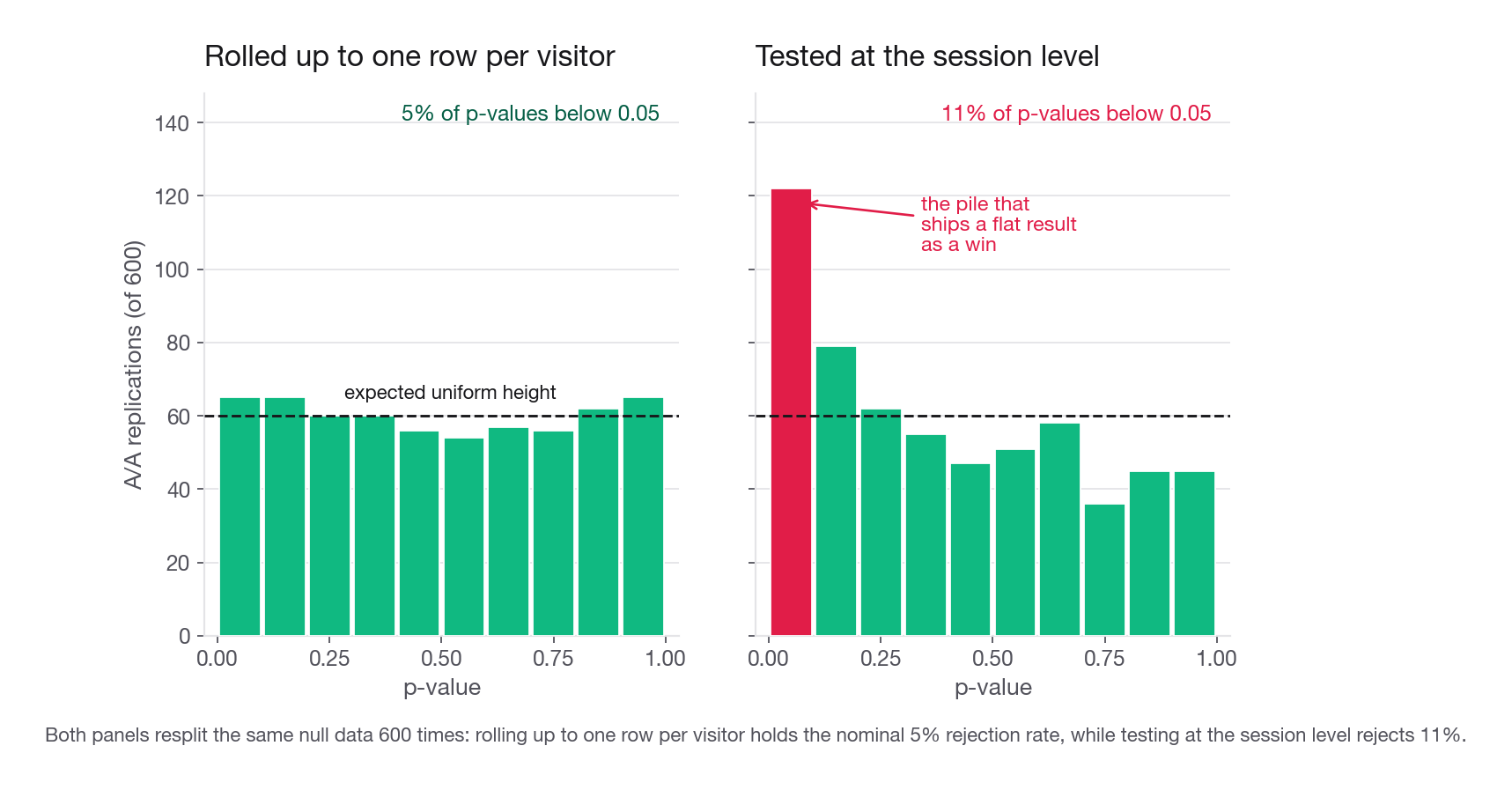
Here is the version that earns its keep. Loomlane assigns per visitor, but an analyst writes the query at the session level because sessions are what the events table holds. Sessions from one visitor are correlated, so the test believes it has far more independent observations than exist.
sim2 = np.random.default_rng(7)
V = 40_000
sessions = sim2.integers(1, 9, V)
theta = sim2.beta(0.6, 7.8, V)
y = (sim2.random(sessions.sum()) < np.repeat(theta, sessions)).astype(int)

flat, rolled = [], []
starts = np.r_[0, np.cumsum(sessions)[:-1]]
per_visitor = np.add.reduceat(y, starts) / sessions
for _ in range(600):
    g = sim2.random(V) < 0.5
    m = np.repeat(g, sessions)
    flat.append(stats.ttest_ind(y[m], y[~m], equal_var=False).pvalue)
    rolled.append(stats.ttest_ind(per_visitor[g], per_visitor[~g], equal_var=False).pvalue)
print(round((np.array(flat) < 0.05).mean(), 3), round((np.array(rolled) < 0.05).mean(), 3))
0.11 0.04Testing at the session level while randomizing at the visitor level rejects a true null 11 percent of the time at a nominal 5 percent. Roll up to one row per visitor and it returns to 4 percent. Every experiment through that pipeline was reported with intervals about a third too narrow, and roughly one flat result in nine shipped as a win. Nothing else in this lesson catches it: the arms are the same size, every covariate balances, exposure is symmetric, and the numbers are wrong anyway.
Interview tip: Say you validate a new metric by resplitting historical data a few hundred times and checking that 5 percent of p-values fall under 0.05. A concrete calibration procedure beats "make sure the test is valid".
Live A/A: when it is worth the traffic
A live A/A routes real traffic through the real assignment service with both arms identical. It is the only check that exercises the platform end to end, and it is expensive, because that traffic is not testing your product. Run one when the platform is new, when the assignment service was rewritten, when you switched identifier, or when a quarter rides on one decision. A permanent one or two percent A/A holdout, split in half and monitored continuously, gives most of the value at fixed cost and turns pipeline drift into an alert instead of a postmortem.
Check four: dilution between assignment and exposure
Assignment happens when a visitor first hits the site. Exposure happens when they land on a category page and see the banner. Those are different moments, and many visitors never reach the second one.
The arithmetic
If a share e of assigned visitors ever encounter the change and the true effect on someone who does is d, the effect measured across everyone assigned is roughly e times d. Visitors who saw nothing contribute zero difference and a full share of variance. Dilution does not bias the intent-to-treat estimate, it shrinks it, and shrinking an effect at fixed sample size destroys power.
exposure = loom.groupby("arm")["reached_listing"].mean()
tab = pd.crosstab(loom["reached_listing"], loom["arm"])
print(exposure.round(4).to_dict(), round(stats.chi2_contingency(tab)[1], 3))

itt_c = loom.loc[loom.arm == "control", "ordered"]
itt_t = loom.loc[loom.arm == "treatment", "ordered"]
res = stats.ttest_ind(itt_t, itt_c, equal_var=False)
print(round(itt_t.mean() - itt_c.mean(), 5), round(res.statistic, 2), f"{res.pvalue:.1e}")
{'control': 0.4374, 'treatment': 0.4397} 0.101
0.00503 6.87 6.3e-12Exposure is 43.74 percent in control and 43.97 percent in treatment, a gap of 0.24 points with a 95 percent interval of about minus 0.05 to plus 0.52. The chi-square returns p equal to 0.101 and the reflex is to call that symmetry. Do not. The mismatch drops about 9 percent of treatment's low-tier rows, and low tier reaches a category page roughly 10 points less often than the others, so removing them raises treatment's exposure rate arithmetically: holding per-tier rates fixed and varying only the tier mix reproduces 0.19 of the observed 0.24 points, about 79 percent of the gap.
So the p-value is not evidence of symmetry, it is a test too weak to see an asymmetry that is provably there: across 900 regenerations the gap averages plus 0.18 points, is positive in 88 percent of them, and still clears the 5 percent line three times in four.
Intent to treat versus exposed only
seen = loom[loom.reached_listing == 1]
c_s, t_s = seen.loc[seen.arm == "control", "ordered"], seen.loc[seen.arm == "treatment", "ordered"]
r_seen = stats.ttest_ind(t_s, c_s, equal_var=False)

miss = loom[loom.reached_listing == 0]
c_m, t_m = miss.loc[miss.arm == "control", "ordered"], miss.loc[miss.arm == "treatment", "ordered"]
r_miss = stats.ttest_ind(t_m, c_m, equal_var=False)

print(len(seen), round(t_s.mean() - c_s.mean(), 5), f"{r_seen.pvalue:.1e}")
print(len(miss), round(t_m.mean() - c_m.mean(), 5), round(r_miss.pvalue, 3))
207593 0.01085 4.1e-21
265799 0.00043 0.645Three numbers to read together. On the 207,593 visitors who reached a category page the banner moves order rate by 1.085 points, a 15.8 percent relative lift. Across everyone assigned the same change is worth 0.503 points, a 7.7 percent lift. On the 265,799 who never reached a category page the difference is 0.043 points at p equal to 0.645. Dividing the intent-to-treat effect by the exposure rate gives 0.0115, close to the 0.0109 measured on the exposed, which checks arithmetic, not correctness. The exposed-only number is contaminated too: across 900 regenerations it averages 1.128 points against a true 1.100 among the exposed, a 0.028-point upward bias from the deleted low-tier rows.
That third number is the part candidates skip and the sharpest tool here. Visitors who never saw the banner cannot have been affected by it. If they show a difference the exposure log is lying: the flag leaked outside the intended surface, the exposure event is not firing where you think, or the arms differ somewhere you did not intend. A significant effect among the unexposed invalidates a readout more decisively than an SRM does.
Interview tip: Propose the unexposed placebo comparison by name. It costs one query, it is a real falsification test, and almost nobody offers it unprompted.
When conditioning on exposure is illegal
Filtering to exposed visitors is defensible only when the exposure rates match, which here they do not quite do. Change the feature slightly and it stops being defensible.
Suppose the treatment also changed the home page so more visitors clicked through. Exposure is now a consequence of the treatment, so filtering on it is filtering on a post-treatment variable. The exposed groups stop being comparable, because treatment's now holds marginal browsers control's never contains, and a randomized comparison has become an observational one whose bias can point either way.
The rule is not "run a test and see whether it clears", the trap the previous section walked into. Report the exposure-rate gap as an estimate with an interval: here 0.24 points, roughly minus 0.05 to plus 0.52. Name the disqualifying gap in the test plan before the experiment starts; if the interval does not exclude it, you have an underpowered result, not a clean one. Default to intent to treat and keep any exposed-only number out of the launch memo.
If the rates do match tightly, conditioning estimates the effect on the exposed under one further assumption: that treatment did not change which people get exposed. Equal rates are evidence for that, not proof, since a treatment can swap who gets exposed while holding the rate fixed. Back it by rerunning check two inside the exposed subsample, the per-variable battery and the adversarial classifier restricted to reached_listing == 1. Keep the unexposed placebo comparison for catching leakage and mis-fired exposure events; it cannot see a reshuffle, because the unexposed pool gets reshuffled in the same motion.
The real fix is where you assign
Dilution is a design problem, not an analysis problem. Assign at the moment of exposure instead of at arrival: the visitor requests a category page, the service assigns them there, and only visitors who could have seen the banner enter the experiment. Exposure goes to 100 percent and the required sample collapses by roughly the square of the old exposure rate.
Trigger-time assignment has its own trap. The trigger must be evaluated identically in both arms, at the same point in the code, before any treatment logic runs. If treatment triggers on "rendered the banner" while control triggers on "loaded the page", control admits everyone and treatment admits only successful renders, and you have manufactured a sample ratio mismatch out of your own instrumentation.
| Design | Exposure | Measured effect | What you are estimating |
|---|---|---|---|
| Assign on arrival, analyse everyone | 43.9 percent | 0.503 points | Effect of launching on all visitors |
| Assign on arrival, analyse exposed | 43.9 percent | 1.085 points | Effect on visitors who reach the surface |
| Assign at the category page | 100 percent | 1.085 points | Same estimate, about five times fewer visitors |
The first two are correct answers to different questions. The launch decision wants the first, because that is the number that reaches the quarterly revenue line. The iteration decision wants the second, because that is what tells you whether the banner design is any good.
Cross-device, logged-out visitors, and shared accounts
Everything so far assumed one row is one person. On a marketplace with heavy logged-out browsing that is wrong for much of the traffic.
A shopper reads reviews on a phone during a commute, then buys on a laptop that evening. If assignment hashes a browser cookie, that is two units, independently assigned, landing in opposite arms about half the time. The human saw both experiences, the phone unit recorded no order, and the laptop unit recorded an order the phone session partly caused. Credit gets scattered across identities, and a contaminated unit experiences a blend of both arms, which pulls the measured difference toward zero.
| Units whose human also appears in the other arm | Attenuation, blended exposure | Attenuation, fully flipped | Extra sample to hold power, blended |
|---|---|---|---|
| 0 percent | 1.00 | 1.00 | 1.0x |
| 5 percent | 0.95 | 0.90 | 1.1x |
| 12 percent | 0.88 | 0.76 | 1.3x |
| 25 percent | 0.75 | 0.50 | 1.8x |
| 40 percent | 0.60 | 0.20 | 2.8x |
At 25 percent contamination a true 1.0 point effect reads as 0.75 and you need 78 percent more traffic to detect it. Nobody notices, because the result is simply weaker than hoped, which is what results usually are.
The responses in order of preference: hash a stable identity such as an account id or a device id surviving reinstall; restrict the test to logged-in visitors when the change sits behind a login anyway, saying plainly that the result generalizes only there; or, stuck with cookies, count accounts appearing under more than one identity and inflate the sample by one over the square of the attenuation. For anything visible and shareable, such as a price, randomize coarser.
Interference between units
The last assumption to break is that one unit's assignment cannot affect another's outcome. On a marketplace it routinely does.
Loomlane's banner promotes listings and sellers hold finite inventory. If treatment buyers clear a maker's stock of hand-dyed scarves, control buyers arrive at a sold-out page. Treatment's lift is then partly a transfer from control rather than new demand, and in a supply-constrained category that can double the apparent effect. The same shape wears several disguises: a promotional budget that treatment drains faster, a ranking model retrained on pooled traffic so control inherits treatment behavior, social features where treatment users invite control users, and two-sided changes that alter what everyone sees.
Detection is indirect, because interference leaves no fingerprint in the assignment log. Three moves work, all of them comparisons against something outside the experiment. Watch control's absolute metric against its own pre-period, since control drifting down while treatment rises is the signature of a transfer. Check whether the effect holds as you ramp, because a real effect stays roughly stable from 10 to 50 percent while an interference-driven one shrinks as the pool of victims shrinks. And measure the constraint itself: sell-out rates and budget exhaustion by arm.
Cluster randomization and market-level designs are the next section's first lesson. What matters here is naming the situation before you present a number rather than after someone else notices.
Interview tip: On a marketplace, a social graph, or anything with shared supply, raise interference yourself in the first minute and say you would ramp to see whether the effect holds. Waiting to be asked reads as not knowing.
Running the checks in order
Two rules make this a gate rather than a ritual. Write the checks and thresholds into the test plan before the experiment starts, so failing one is a pre-agreed stop and not a negotiation. And run them on every experiment, including the flat ones, because a pipeline bug found on a boring test is free and the same bug found on a launch decision is not.
Common traps
Treating an SRM as a rounding error. A 1.2 percent shortfall on half a million rows is a mechanism, not noise, and it usually deletes low-converting sessions. Fix: quote the row deficit and the p-value together, and treat p below 0.001 as blocking. Subsampling the larger arm to match only hides it.
Using a 0.1 standardized-difference rule to clear balance. That threshold was built for observational work, and here it waved through the 0.043 imbalance that was the bug. Fix: test against the null of exact balance, not an effect-size threshold.
Calling an adversarial AUC of 0.51 a null result. On this sample it corresponds to a fifteen-sigma imbalance, and one-hot encoding with drop_first can hide the broken category entirely. Fix: keep every level, and judge the AUC against the null of 0.5 rather than against your intuition about what a good model looks like.
Filtering to exposed visitors without checking exposure symmetry. If the treatment changed who gets exposed, the filter conditions on a post-treatment variable and the comparison stops being randomized. Fix: report the gap with an interval, not a p-value, rerun balance inside the exposed subsample, and default to intent to treat unless both are clean. A non-significant gap from an underpowered test is not symmetry.
Skipping the placebo check on the unexposed. One query catches flag leakage, mis-fired exposure events, and cross-arm contamination. Fix: run it every time and report it.
Analysing sessions while randomizing visitors. The false positive rate more than doubled above, to 11 percent, and nothing else in the checklist notices. Fix: aggregate to the randomization unit, or cluster the variance estimator on it.
Reusing one salt across experiments. Overlapping tests become perfectly confounded and both readouts are meaningless. Fix: put a unique experiment key inside the hashed string, and check that any two live experiments agree at chance.
Assuming the assignment log is ground truth. It is written by the same client that has the bug, so a log that loses treatment rows still looks internally consistent. Fix: reconcile against something outside the experiment, such as server request counts.
Reporting a diluted effect as the effect of the feature. Saying the banner lifts orders 7.7 percent when it lifts them 15.8 percent among people who see it will get the feature killed. Fix: report both, and state which population each number describes.
Ignoring interference because the assignment checks passed. Every check here is about assignment; interference breaks the outcome side instead. Fix: name it whenever supply, budget, a shared model, or a social graph connects the units.
Quick self-check
Answer these aloud, in full sentences, as if the interviewer just asked.
Walk from identifier to arm through the assignment mechanism, and say what the salt does and what breaks when two experiments share one.
Your arms are 239,670 and 233,722 against a designed even split. What do you check next, in what order, and what do you tell the PM meanwhile?
A variable's standardized difference is 0.04 and its chi-square p-value is 1e-40. Which number do you act on, and why does the answer turn on randomization rather than on sample size?
Exposure is 44 percent in control and 51 percent in treatment. What can you no longer estimate, what can you still estimate, and what changes before you rerun?
A pre-period A/A returns 11 percent of p-values below 0.05. Name three causes and how you would tell them apart.
A promoted-listing test shows a 12 percent lift. Give two reasons the launched effect could be materially smaller, and one measurement that says which applies.