3.4 Fraud Detection: Model and Product Design
Find the core decision, design, or behavior signal.
Turn the lesson into a concise response blueprint.
Name the trap you would avoid in a real interview.
Use these checkpoints as your reading path before diving into the full lesson.
- 1Why this matters in interviews
- 2A marketplace table to argue over
- 3What fraud actually leaves behind
- 4Things that are supposed to be unique a...
- 5Things that are extreme, and things tha...
Almost every fraud question in a product loop asks one thing: what does the product do with a number between zero and one that you do not fully trust. Candidates answer the classifier half well and the product half badly, tuning a threshold, quoting an AUC, and stopping. This lesson gets you to the answer a fraud team would recognise: what the score is for, who pays when it is wrong, why the offline number is inflated, and what you build so the attacker's next move does not silently break you.
Why this matters in interviews
Fraud comes up constantly because it compresses four skills into one prompt: inventing features for an adversarial process, reasoning about asymmetric costs, knowing that a random split is dishonest here, and designing an intervention that is not just a block button. Most candidates handle the first and lose the room on the other three.
Here is the weak answer: "I would build a gradient boosted model, use recall because missing fraud is expensive, and pick the threshold where recall is highest subject to acceptable precision." Nothing there is wrong. Nothing is worth anything either. It names no cost, says nothing about who reviews the flagged cases, does not admit the labels are partly fiction, and treats the product as a switch with two positions.
The stronger version starts elsewhere. "A fraudulent listing costs us about 180 dollars once you count the buyer refund, the card network fee, and the support contact. Wrongly stopping a legitimate listing costs about 60 dollars in forward margin. That three to one ratio puts my break-even probability at 0.25. But before I pick a threshold I want a third option, because there is a wide band where blocking is too aggressive and allowing is too generous, and in that band an identity check earns more than either." Now you are having a design conversation.
Interview tip: Say the two costs out loud, in currency, in your first ninety seconds. Everything else in a fraud answer is downstream of that ratio, and interviewers grade you on whether you reached for it unprompted.
Two fictional products carry the examples. Kestrel is a peer to peer marketplace for used camera and audio gear, where the fraud is fake listings: an account posts gear it does not have, takes payment, and disappears. Trailhead is a professional network, where the fraud is fabricated credentials. The two look unrelated and share almost all of their structure.
A marketplace table to argue over
Everything below runs on one synthetic Kestrel listing table. Each row is a listing at publish time, holding only what the platform could see that day, plus two label columns whose difference is the point of the label section later. A few percent of honest sellers share a household device, so sharing is suggestive rather than conclusive. Deterministic, numpy and pandas only.
import numpy as np
import pandas as pd

SEED = 20260826
rng = np.random.default_rng(SEED)
N_SELLERS, N_RINGS, HORIZON = 20_000, 24, 180

ring_seller = rng.random(N_SELLERS) < 0.010
ring_of = np.where(ring_seller, rng.integers(0, N_RINGS, N_SELLERS), -1)
ring_start = np.sort(rng.integers(5, HORIZON - 20, N_RINGS))
adapt = ring_start / HORIZON               # later rings have studied our detectors
joined = np.where(ring_seller, ring_start[ring_of] + rng.integers(0, 3, N_SELLERS),
                  rng.integers(0, HORIZON - 10, N_SELLERS))
n_list = np.where(ring_seller, rng.poisson(4.0, N_SELLERS), rng.poisson(1.4, N_SELLERS)) + 1

sid = np.repeat(np.arange(N_SELLERS), n_list)
bad, n = ring_seller[sid], sid.size
a = np.where(bad, adapt[ring_of[sid]], 0.0)
day = np.clip(joined[sid] + np.where(bad, rng.integers(0, 3, n),
                                     rng.exponential(22.0, n).astype(int)), 0, HORIZON - 1)
age = np.clip(day - joined[sid], 0, None)
sus = np.where(bad, rng.normal(1.45, 1.05, n), rng.normal(0.0, 1.0, n)) - a
pool = 1 + np.round(adapt[np.clip(ring_of[sid], 0, None)] * 9).astype(int)

kestrel = pd.DataFrame({
    "listing_id": np.arange(n), "seller_id": sid, "ring_id": ring_of[sid],
    "device_id": np.where(bad, 10_000_000 + ring_of[sid] * 100 + sid % pool, sid),
    "day": day, "acct_age_days": age,
    "price_vs_category_median": np.clip(rng.normal(1.0 - 0.19 * sus, 0.29, n), 0.05, None).round(3),
    "photo_reverse_match": (1 / (1 + np.exp(-(-1.7 + 0.62 * sus + 0.7 * bad * (1 - a)
                                              + rng.normal(0, 0.8, n))))).round(3),
    "duplicate_desc_count": rng.poisson(np.exp(-2.1 + 0.52 * sus + 0.8 * bad * (1 - a))),
    "browse_minutes_pre_listing": np.exp(rng.normal(3.0 - 0.50 * sus, 0.95, n)).round(1),
    "seller_rating_count": rng.poisson(np.clip(0.09 * age * (1 - 0.75 * bad), 0, None)),
    "is_fraud": bad.astype(int)})
kestrel["confirmed_fraud"] = (bad & (day <= HORIZON - 45) & (rng.random(n) < 0.72)).astype(int)

hh = np.flatnonzero(~ring_seller & (rng.random(N_SELLERS) < 0.03))  # honest device sharing
share_to = hh[rng.integers(0, max(hh.size // 3, 1), hh.size)]       # households of about three
dev_map = np.arange(N_SELLERS); dev_map[hh] = share_to
kestrel.loc[~bad, "device_id"] = dev_map[sid[~bad]]
That produces 48,719 listings from 20,000 sellers over 180 days. 963 are fraudulent, a base rate of 1.98 percent, from just 190 seller accounts organised into 24 rings. Only 613 of the 963 are ever confirmed, which is the most important number on this page.
| Column | What it is | Why a fraud team cares |
|---|---|---|
device_id | Device fingerprint at publish time | Rings reuse hardware, so this joins accounts that claim to be strangers |
acct_age_days | Days from signup to this listing | Rings list immediately, real sellers usually browse first |
price_vs_category_median | Asking price over the category median | Underpricing is how a fake listing gets bought fast |
photo_reverse_match | Similarity of the photo to an image found elsewhere online | Stolen photography, but legitimate resellers use stock shots too |
duplicate_desc_count | Other live listings with near identical copy | Copy and paste at volume |
browse_minutes_pre_listing | Session minutes before publishing | Real first time sellers explore, scripted accounts do not |
seller_rating_count | Completed sales with feedback | Reputation is expensive to fake and cheap to check |
is_fraud | Ground truth, available only inside the simulation | Used here to grade honestly, never available in production |
confirmed_fraud | What the operations queue actually recorded | The only label you may train on |
Read the last two rows again. In production you hold confirmed_fraud and you pretend it is is_fraud. That gap is where most fraud modelling goes wrong, and we return to it once the easier parts are settled.
What fraud actually leaves behind
Three ideas generate almost every useful fraud feature, and stating them cleanly lets you invent features live for any product you are handed.
Things that are supposed to be unique and are not
Fraud at any scale needs many identities. One fake listing is not a business, forty are. But the attacker does not have forty phones, forty bank accounts, or forty payment cards, because acquiring those honestly is the expensive part. So they reuse, and every field meant to identify exactly one person becomes a join key that stitches the fake accounts back together: device fingerprint, browser and font profile, network address, payout account, card issuer and last four digits, normalised shipping address, phone number, even the pixel dimensions of an uploaded photo.
In the Kestrel table, 88 percent of fraudulent listings sit on a device carrying at least one other confirmed fraud, and the median fraudulent listing's device has served three distinct seller accounts against one for legitimate listings. That is the strongest raw signal on the platform and it is nearly free to compute. Marketplace fraud interviews often turn into a SQL question, so here is the shape of it.
SELECT l.listing_id,
       COUNT(DISTINCT CASE WHEN p.seller_id <> l.seller_id
                           THEN p.seller_id END)             AS other_accounts_on_device,
       SUM(CASE WHEN p.confirmed_fraud = 1
                 AND p.day <= l.day - 45 THEN 1 ELSE 0 END)  AS prior_bad_on_device
FROM listings AS l
LEFT JOIN listings AS p
  ON p.device_id = l.device_id
 AND p.day < l.day                -- the device graph itself is visible instantly
GROUP BY l.listing_id;
Three details there are the whole exam. It is a LEFT JOIN: an inner join deletes every listing whose device has no earlier row, exactly the population the feature exists to catch, and the inner version returns 3,447 rows of 48,719 with no fraudulent listing among them. The p.seller_id <> l.seller_id case stops the seller being counted against themselves. And the 45 day predicate sits inside the prior_bad_on_device sum alone, because only that column is label derived. Watching which accounts touch a device needs no review decision, so that count carries no lag.
Things that are extreme, and things that are too fast
The second idea is that fraud is a tiny minority behaving unusually, so distribution tails carry information. But the useful version of "extreme" is about rate, not level. Ten listings is not suspicious. Ten listings in nine minutes from an account opened this morning is. Velocity features, counts per unit time per entity, beat static counts in nearly every fraud system, and candidates forget them entirely.
The third family is behavioural realism. A genuine first time seller browses comparables, opens help pages, abandons the listing form once. The median legitimate listing here follows about 20 minutes of session time, while a scripted account goes straight from signup to publish. Attackers optimise for throughput and humans do not.
The listing side and the seller side
For any marketplace prompt, split the brainstorm into the thing being sold and the person selling it. It keeps you organised out loud and matches how the platform is instrumented.
| Angle | Listing side features | Seller side features |
|---|---|---|
| Uniqueness violation | Photo matches an image already on the web, description duplicated across listings, identical serial numbers | Device, payout account, address, and phone shared with other sellers |
| Extremes | Price far under the category median, unusually high quantity, shipping promised faster than physically possible | Listings per hour, messages per hour, account age in hours at first listing |
| Behavioural realism | Description missing details a real owner would know, no original photo angles | Time on site before signup, help pages viewed, form abandoned and resumed |
| Reputation | Category the seller has never sold in before | Completed sales, feedback count, months since first sale |
Interview tip: When asked for fraud features, do not list twenty items. Name the three generators, uniqueness violated, extremes and velocity, behavioural realism, then produce four features from each. Interviewers score the framework, not the length of the list.
Fake profiles: the network is the evidence
The Trailhead version looks different and is not. A member claims a degree from a university they never attended. You cannot check that directly without verified institutional email, and asking everyone is a bad product: most honest members will not bother, so you trade a fraud problem for a coverage problem where most true credentials go unverified.
The move is to stop evaluating the claim and start evaluating the graph around it. Typing a university name takes four seconds. Building a connection graph that resembles someone who spent four years there takes months of coordinated work. For members claiming a given school and year, compare their connection pattern with that of members whose credential is already verified:
Overlap: how many of their connections claim the same school and years, versus the typical verified member
Reciprocity: the acceptance rate on invitations they sent to alumni of that school, since a stranger blasting invitations gets refused far more often
Triangles: whether their alumni connections know each other, because real classmates form dense clusters and randomly harvested ones do not
Sequence: whether they viewed a profile before connecting, which is what a person remembering a classmate does
Run this as an outlier problem within the claimed cohort, not as a global classifier. Two shapes matter: small tight clusters behaving the same odd way, which is a credential mill, and isolated points far from every legitimate cluster, which is one person embellishing. The payoff is that you demand verification only from the few percent whose graph does not hold up, the same intervention at one twentieth of the friction.
That last pair is where models die quietly. A feature such as account_status will be the strongest predictor in the model and exists only because a human already decided the case. You find out the week after launch, when live performance is a third of what the notebook promised.
Cost asymmetry, in currency, before anything else
Fraud is the canonical asymmetric cost problem, though the asymmetry is not always in the direction people assume. For Kestrel, take these numbers as agreed with finance and support:
| Outcome | What happens | Cost |
|---|---|---|
| Fraud allowed through | Buyer refunded, card network fee, support handling, some churn from the burned buyer | 180 per listing |
| Legitimate listing stopped | Forward margin lost from that seller, support contact, some never return | 60 per listing stopped |
| Fraud correctly stopped | Ring loses a mule account, small review cost | About 0 |
| Legitimate seller allowed | The product working | 0 |
The break-even probability falls straight out. Blocking wins when the expected loss from allowing exceeds the expected loss from blocking: p * 180 > (1 - p) * 60, so p > 60 / (180 + 60) = 0.25. Score above 0.25, stop it; below, let it through. That is the whole content of choosing a threshold, and the unbalanced classes lesson earlier in this section derives the same thing from the cost matrix side.
Two things candidates get wrong. First, treating the fraud cost as the transaction value. It is the refund plus the fee plus the support time plus the damage to the burned buyer's willingness to transact again, and that last term is usually the largest. Second, quoting a lifetime value of several hundred dollars for a blocked seller because a growth slide says so. The relevant quantity is the incremental margin lost from this seller onward, discounted, times the probability they do not appeal and get reinstated. Appeals recover a good share of false positives, which cuts the effective cost and licenses a tighter policy.
Say the unit out loud: this table charges 60 per listing decision. Enforce per account instead and friction is charged once per seller, 0.06 times 9,671 sellers times 60 on this window, so 34,816 rather than 71,536. Universal friction still loses, by less.
Interview tip: If you are asked for a case where a false positive costs more than a false negative, do not reach for a medical example. Say content moderation on a creator platform: wrongly removing a top creator's video costs more reach, trust, and press than leaving one borderline video up for six hours.
The third lane: step-up authentication
Now the part that separates levels. Allow or block forces the whole cost asymmetry through one threshold. Real systems have a middle option: make the user prove something. On Kestrel that is an identity check before the listing goes live, elsewhere a one time code, a card verification, a payout hold. It is worth modelling explicitly because it changes both costs: it does not stop all fraud, and it does not cost a full wrongful block. Two parameters:
A step-up stops about 70 percent of fraud attempts that hit it, because rings will not burn a real identity document on a mule account
About 6 percent of honest sellers abandon rather than complete it, and each abandonment costs the same 60 as a wrongful block
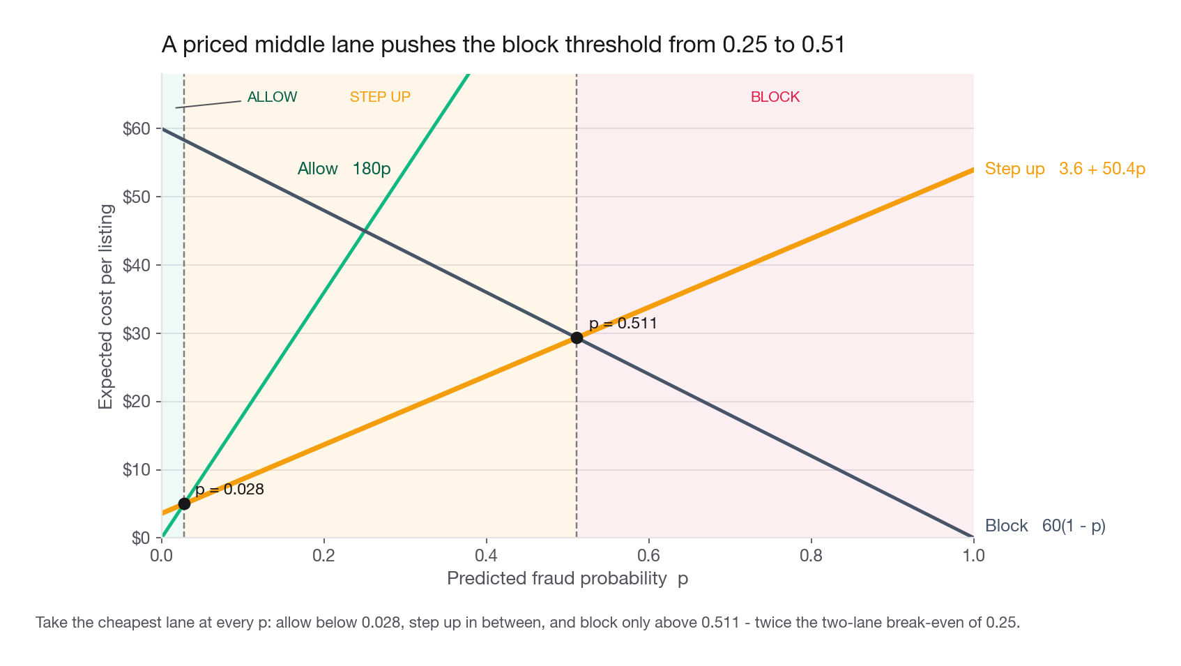
Write the expected cost per listing for each lane as a function of the model's probability p:
| Lane | Expected cost | At p = 0.01 | At p = 0.20 |
|---|---|---|---|
| Allow | 180p | 1.80 | 36.00 |
| Step up | 3.6(1 - p) + 54p | 4.10 | 13.68 |
| Block | 60(1 - p) | 59.40 | 48.00 |
Setting the lines equal gives both boundaries. Allow beats step-up while 180p < 3.6 + 50.4p, so below p = 0.028. Step-up beats block while 3.6 + 50.4p < 60 - 60p, so below p = 0.511. The policy: allow under 0.028, step up between, block above 0.511.
Look at what happened to the block threshold: 0.25 with two lanes, 0.51 with three. A cheap middle option does not merely fill a gap, it makes blocking twice as hard to justify, because there is now something better to do with a moderately risky user.
LOSS, GOOD, STEP_STOPS, ABANDON = 180.0, 60.0, 0.70, 0.06

def lane_costs(p):
    return {"allow": LOSS * p,
            "step_up": ABANDON * GOOD * (1 - p) + LOSS * p * (1 - STEP_STOPS),
            "block": GOOD * (1 - p)}

def boundaries():
    lo = ABANDON * GOOD / (LOSS - LOSS * (1 - STEP_STOPS) + ABANDON * GOOD)
    hi = (GOOD - ABANDON * GOOD) / (GOOD + LOSS * (1 - STEP_STOPS) - ABANDON * GOOD)
    return round(lo, 3), round(hi, 3)

print(boundaries())
print({k: round(v, 2) for k, v in lane_costs(0.20).items()})
(0.028, 0.511)
{'allow': 36.0, 'step_up': 13.68, 'block': 48.0}What the lanes are worth
Train the honest model from the next section on days 0 to 119 and apply the policy to days 120 to 179, a window of 20,082 listings of which 211 are fraudulent, a rate of 1.05 percent.
| Policy | Listings affected | Fraud caught | Net saved over 60 days |
|---|---|---|---|
| Do nothing | 0 | 0 | 0, and 37,980 lost |
| Best possible allow or block threshold | 167 blocked at 0.443 | 119 | 18,540 |
| Three lanes at 0.028 and 0.511 | 470 stepped up, 163 blocked | 49 stepped, 117 blocked | 22,958 |
| Step up every listing | 20,082 | 148 | negative 44,950 |
Three lanes beat the best two lane policy by about a quarter, 22,958 against 18,540, while checking everyone destroys about 45,000 dollars in the same window, because 6 percent abandonment across 19,871 honest listings, from 9,671 distinct sellers, swamps everything caught. Memorise the mechanism, not the multiple: the third lane earns most when the score is mediocre and the risk sits in the ambiguous middle, least when the model separates cleanly and the middle thins out, here to 470 listings. The last row holds however good the model is. Universal friction loses because the honest population is 99 percent of the traffic and pays the whole cost.
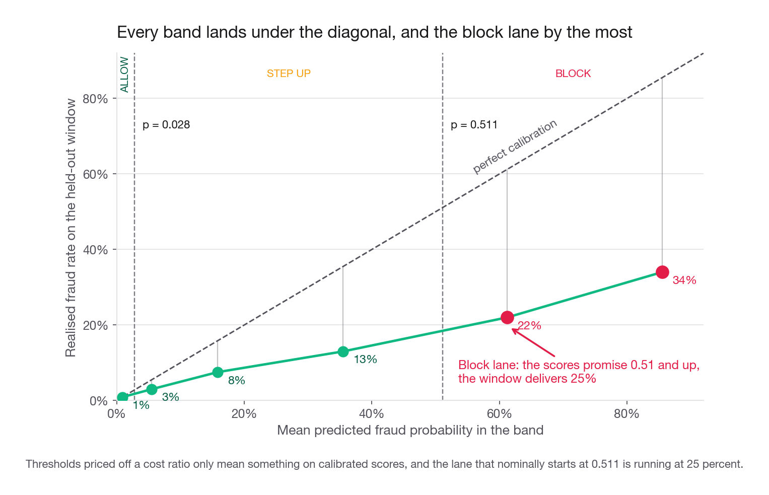
Now check the block column against its own promise. The 163 blocked listings carry a mean predicted probability of 0.88 and a realised fraud rate of 0.72, and the band below is overconfident too: scores between 0.2 and 0.511 predict 0.30 and deliver 0.20. A threshold from a cost ratio is only valid on calibrated scores, so that gap matters, but here it does not flip the decision: 0.72 sits far above the 0.25 break-even and the lane nets 18,300. You only know that because you measured it. Report the realised rate beside the nominal one, and do not read a weak realised precision as miscalibration when a missing feature explains it better.
Interview tip: After you derive a threshold from costs, add one sentence: "and I would check the realised rate in the region of the threshold, because a lane that scores 0.88 and delivers 0.72 is still worth blocking, while one that scores 0.51 and delivers 0.20 is not, and the ranking metric cannot tell those apart."
How you would actually prove it works
Do not evaluate step-up by switching it on and watching fraud fall: losses arrive with a lag and drift on their own, so that comparison is uninterpretable. Randomise inside the risky band instead. Among listings scoring between 0.028 and 0.511, send 90 percent to the identity check and let 10 percent through. That holdout measures the band's true fraud rate, which tells you whether your probabilities are honest, prices abandonment cleanly, and keeps producing labels where the model most needs them.
Size it: at 470 listings per 60 days in the band and a 10.4 percent fraud rate, a 10 percent holdout yields about 47 listings and 5 frauds. That is far too thin to price the band, so either widen it to 25 percent, which buys 118 listings and 12 frauds a quarter, or pool several quarters before you quote a number, and say which you chose.
Why a random split lies about fraud
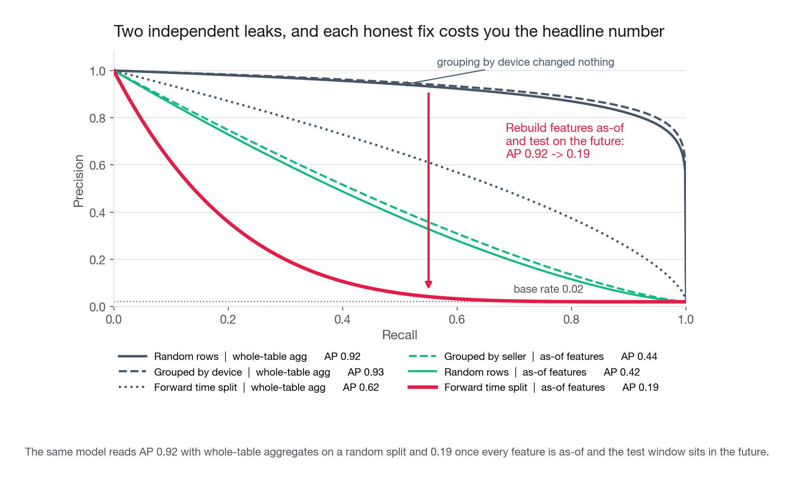
Here is the number that should make you suspicious of your own notebook. Fit the model with device history aggregated over the whole table, split rows at random, and average precision is 0.92 against a 2 percent base rate. Restrict features to what was available at decision time, train on the first 120 days, test on the last 60, and it is 0.19. Three quarters of the headline was artefact, from two independent mistakes, and candidates usually know about one. Part of that collapse is recoverable and part is not, and separating them is the step almost nobody takes.
Mistake one: the feature was computed with information from the future
dev_frauds_all_time counts confirmed frauds on a device across the whole table, so a listing on day 30 carries frauds confirmed on day 150. Worse, confirmation lands about 45 days after the event, so even the earlier frauds were unknown on day 30. Both problems live in the feature, not the split.
The as-of version answers a stricter question: what had review settled by the day this listing went live. pandas.merge_asof says it directly.
REVIEW_LAG = 45

known = (kestrel.query("confirmed_fraud == 1")
         .assign(known_day=lambda d: d["day"] + REVIEW_LAG)
         .groupby(["device_id", "known_day"]).size()
         .groupby(level=0).cumsum()
         .rename("dev_frauds_asof").reset_index().sort_values("known_day"))

kestrel = pd.merge_asof(kestrel.sort_values("day"), known,
                        left_on="day", right_on="known_day",
                        by="device_id", direction="backward")
kestrel["dev_frauds_asof"] = kestrel["dev_frauds_asof"].fillna(0)
kestrel = kestrel.sort_values("listing_id").reset_index(drop=True)
Run it on Kestrel and the as-of count is zero for every row in the table, not merely the fraudulent ones. Not small: zero, everywhere, all 48,719 rows. A ring here runs its listings inside about four days against a 45 day review lag, so no confirmation lands before the campaign it belongs to has finished. The column is constant, so the model carrying it is bit for bit the model with no device feature at all.
This is where a candidate overclaims, so be careful. What died is the label derived count, not the device, and how hard the lag bites depends on ring speed against your confirmation cycle, so do not turn one simulation into a law about marketplace fraud. The device graph itself needs no review decision: which accounts touched a piece of hardware is visible the moment the listing publishes. Build that, from strictly earlier days, the same quantity the SQL computes.
d = kestrel[["device_id", "day", "seller_id"]]
first_seen = d.groupby(["device_id", "seller_id"])["day"].min().rename("self_first").reset_index()
new_acct = (first_seen.groupby(["device_id", "self_first"]).size()
            .rename("na").rename_axis(["device_id", "day"]).reset_index())
per = (d.groupby(["device_id", "day"]).size().rename("nl").reset_index()
       .merge(new_acct, on=["device_id", "day"], how="left").fillna(0)
       .sort_values(["device_id", "day"]))
per["dev_listings_prior"] = per.groupby("device_id")["nl"].cumsum() - per["nl"]
per["acct_prior"] = per.groupby("device_id")["na"].cumsum() - per["na"]

kestrel = (kestrel.merge(per[["device_id", "day", "dev_listings_prior", "acct_prior"]],
                         on=["device_id", "day"], how="left")
                  .merge(first_seen, on=["device_id", "seller_id"], how="left"))
kestrel["dev_other_accounts_prior"] = (kestrel["acct_prior"]
    - (kestrel["self_first"] < kestrel["day"]).astype(int)).clip(lower=0)
Those two columns fire on 58 and 76 percent of fraudulent listings against 2 and 58 percent of legitimate ones. Add them to the honest feature set, keep the same forward split, and average precision goes from 0.19 to 0.59 with AUC at 0.99. The split did not change, so this is not a leakage fix. The lesson is narrower and far more useful than "the device signal is gone": the label derived version of a graph feature inherits your review lag, the label free version does not, and swapping one for the other is most of the work. Say the caveat too: honest sellers share devices here at only 3 percent, and with that removed every shared device is fraudulent by construction and the count is an oracle, not a feature. Real sharing is messier, so 0.59 flatters. Defend the direction, not the decimal.
Mistake two: the split does not resemble deployment
Even with honest features, a random row split flatters you. Deployment means predicting a period you have not seen, against attackers who have watched three months of your enforcement. On Kestrel, later rings use more devices and recycle fewer photographs: among fraudulent listings in the first 90 days, mean photo_reverse_match is 0.41 and mean duplicate_desc_count is 0.45, falling to 0.30 and 0.25 in the last 90 days against a legitimate baseline near 0.20. A random split hides that by mixing the adapted rings into training.
| Split | Feature construction | Average precision |
|---|---|---|
| Random rows | Device aggregates over the whole table | 0.92 |
| Grouped by device | Device aggregates over the whole table | 0.93 |
| Train days 0 to 119, test 120 to 179 | Device aggregates over the whole table | 0.62 |
| Random rows | As-of features only | 0.42 |
| Grouped by seller | As-of features only | 0.44 |
| Train days 0 to 119, test 120 to 179 | As-of features only | 0.19 |
| Train days 0 to 119, test 120 to 179 | As-of features plus label free device counts | 0.59 |
Read the second row carefully, because it kills a common half-measure. Grouping by device so that none appears on both sides bought nothing: 0.92 became 0.93. The leak lived inside the feature, computed over the full table before any split existed. Entity grouping protects you when the same entity's rows straddle the boundary and does nothing when the feature itself peeked. The two fixes are independent and you need both.
Row five deserves a note. Grouping by seller moved the honest number from 0.42 to 0.44, essentially nothing, because in that feature set each listing's features are drawn per listing rather than shared. Row seven is the counterexample: its device counts are shared across every row on the device, so a device grouped split becomes a live control there. Entity splits matter exactly as much as your features are shared across rows of the same entity, no more and no less.
The split I would actually propose
State it as a recipe and interviewers stop probing:
Order by event time and cut forward: train on an early window, validate on the next window, test on the most recent window.
Embargo the tail of training by the review lag. Rows from the last 45 days have immature labels; treat them as unlabelled rather than as negative.
Hold out whole entities where features are entity level: no device, payout account, or ring split across the boundary.
Rebuild every aggregate feature as-of each row's own timestamp, from a point in time store or a windowed join, never a global groupby.
Report the metric your operations team lives with, not average precision, which appears here only because it compresses the comparison.
Interview tip: When asked how you would split the data for fraud, answer with three words before any detail: time, entity, and label maturity. Most candidates offer one of the three, and naming all three signals you have shipped something.
The label you train on is not the label you want
The Kestrel table holds 963 fraudulent listings and 613 confirmations, so 350 genuine frauds, 36 percent, sit in the data labelled zero. That is the defining property of fraud data, with three consequences a strong candidate raises unprompted.
First, the model is actively taught that undetected fraud is fine: whatever technique evaded detection now sits reinforced in the negative class. The better an attack is, the harder your training set argues it is legitimate, and the loop tightens the longer it runs.
Second, measured precision is pessimistic and measured recall is unknowable, because a label set that missed a third of fraud will score some correct catches as mistakes. Never report precision from confirmed labels without saying the denominator is incomplete.
Third, enforcement censors its own evidence. Once you block an account you never learn whether it would have defrauded anyone, so every block is a destroyed counterfactual. Run that for a year with no randomised release and you cannot answer the first question a director asks, which is how much of what we block is actually bad.
The fix is cheap and rarely done: release a small random sample of the highest scoring cases, watch them closely, and book the losses as measurement cost. Size it before you propose it, because a token release buys nothing. Kestrel's block lane is 163 listings per 60 days at a realised precision of 0.72, so a 2 percent release is three listings a quarter and tells you nothing. Cost is released listings times realised precision times 180. Release a tenth of the lane, 16 listings, and you lose 16 times 0.72 times 180, about 2,100 per 60 days, or 246 a week, against the 22,958 the policy saves. Sixteen outcomes a quarter is thin, so pool a year or release a quarter of the lane at about 615 a week. Have the multiplication ready, not just the number.
Supervised, unsupervised, or both
The classic prompt asks what goes wrong if you treat fraud as ordinary supervised learning. Everything above is part of the answer. The rest is structural.
Supervised models learn the frauds you already caught, which is genuinely useful because most fraud volume is repetition: an attack that works gets run thousands of times, so last month's confirmed cases cover most of next month's volume. What such a model cannot do is recognise a technique absent from its training data, and the highest value attacks are exactly the novel ones. You stay one cycle behind: the ring innovates, extracts money for weeks, you confirm the losses, you retrain, and the ring has already moved.
Anomaly methods flip the assumption: instead of asking whether this looks like known fraud, ask whether it looks like anything you normally see. That covers novel attacks and needs no labels, which matters when you hold 613 positives in total. The price is precision. In high dimensions almost every record is unusual on some axis, so a naive detector floods the review queue. Making it work is the unglamorous labour of picking a small, well understood feature space and defining normal per segment, because a listing that is anomalous for a hobbyist is routine for a professional dealer.
The senior answer is that these are layers, not options. Run the supervised model for volume, run anomaly detection over the segments it scores safe, keep a rules layer for incidents with a mandatory review date, and use graph linking to expand from any confirmed bad account to its neighbours. Block when the model is confident or the account is one hop from a confirmed ring, step up when either signal is moderate. That degrades gracefully: defeat one layer and another still fires.
The adversarial loop, and designing for it
Everything in a fraud system decays, because a person on the other side is reading your responses. Train once on days 0 to 119 and evaluate on successive 20 day windows: average precision runs 0.642, then 0.609, then 0.457. Nothing broke. The model aged against a moving opponent.
Three design choices follow, and they are worth your last two minutes in an interview.
Retrain on a schedule shorter than the attack cycle and hold it even when metrics look fine. Weekly retraining on a rolling two year window is normal, and automatic deployment matters more than frequency: a model waiting for a human to notice decay is always one incident behind.
Monitor inputs, not just outcomes. Outcome metrics arrive 45 days late and cannot alert you, while feature distributions arrive instantly. Track the share of listings above each threshold, the daily mean of every top feature, and the fraction of new sellers on a device already seen this week. A tactic switch shows up as a distribution shift weeks before it shows up as a loss.
Keep information channels the attacker cannot poison. The random release holdout is one. Rate limited enforcement is another: blocking instantly and identically every time hands the ring a fast, free oracle telling them exactly which change worked. Jitter, daily batched sweeps, and varying the response between block and step-up all raise the cost of probing. The counterintuitive part lands well in an interview: a slower, noisier enforcement policy can catch more fraud over a quarter than an instant one, because it denies the adversary a clean feedback signal.
Reporting the model to people who are not you
Report the number operations lives inside, and get the unit right, because a queue is a daily thing and depth in a pooled ranking is not. Kestrel's test window runs about 335 listings and 3.5 frauds a day, so the constraint is twenty to forty cases a day. At the daily top 20 the model reaches 80 percent of fraud at 14 percent precision, so roughly 3 of every 20 cases a reviewer opens are genuinely bad; widen to 40 a day and recall goes to 97 percent at 8.5 percent precision. That beats quoting an average precision of 0.59, and it avoids the classic slip of reporting the top 200 of a pooled 60 day ranking as a daily capacity.
| Metric | Question it answers | Where it misleads |
|---|---|---|
| AUC | Does the score rank a random bad case above a random good one | Sat near 0.97 on the as-of model even after its useful range collapsed, because 98 percent of pairs are easy |
| Average precision | How good is the whole ranking against the base rate | Not a decision, and moves with the base rate so it is not comparable across periods |
| Recall at review capacity | What share of fraud does today's team actually reach | Depends on staffing, so restate it whenever capacity changes |
| Value weighted recall | What share of fraud losses, in currency, do we prevent | Needs a per case loss estimate, which finance may dispute |
| False positive rate on good sellers | How much of the honest population do we inconvenience | A tiny rate on a large denominator is still a lot of angry people |
| Realised precision by score band | Are the probabilities honest where we make decisions | Needs the random release holdout to be unbiased |
If you present one chart, make it the last row: predicted probability band against realised fraud rate, with the lane boundaries drawn on. It carries ranking quality, calibration, and policy in one picture, and it is the chart a fraud lead keeps.
Common traps
Optimising one threshold when a third lane exists. Price the middle intervention explicitly. Adding step-up moved Kestrel's block threshold from 0.25 to 0.51 and added about a quarter to the policy's value, far more when the model ranks poorly.
Treating confirmed fraud as truth. A third of real fraud sits in the negative class. Say so, and name the response: positive and unlabelled framing, a random release holdout, and never reporting precision without flagging the incomplete denominator.
Random train and test splits. Fraud is bursty, organised, adversarial, and late labelled. Split forward in time, hold out whole entities where features are entity level, and embargo the immature tail.
Aggregate features built with a global groupby. A device fraud history computed over the whole table leaks the future into every row and no split repairs it. Build every aggregate as-of the row's own timestamp, and subtract the review lag only from the label derived ones. Lagging a device account count as well is how a usable feature gets thrown away.
Features downstream of enforcement. Case notes, review flags, account status, anything a human touched after the decision. They dominate offline and are useless online.
Quoting accuracy, or celebrating an AUC of 0.97. At a 2 percent base rate, calling everything legitimate scores 98 percent accuracy. AUC sat at 0.97 across the as-of splits while average precision fell from 0.42 to 0.19.
Assuming the score is calibrated. Thresholds derived from a cost ratio are only meaningful on calibrated probabilities. Kestrel's block lane averages 0.88 and delivers 0.72, still a correct block, and the only way you learn that is by measuring the realised rate in the band instead of trusting the score.
Universal friction as a fraud fix. Verifying every listing loses about 45,000 dollars per 60 days on this traffic. The honest population is the denominator, and friction is charged to all of it.
Instant, deterministic enforcement. It hands the attacker a free oracle. Batch it, jitter it, and vary the response.
Forgetting the appeal path. Every wrongly stopped seller needs a route back, because it is the right product call and because it lowers the effective cost of stopping someone, which licenses a tighter policy.
Quick self-check
Answer each out loud, in under a minute, without notes.
State the two costs for a fraud problem on any product you know, in currency, and derive the break-even probability from them. Then say how that threshold moves once you add a step-up lane.
Explain in three sentences why a random train and test split overstates fraud model performance, naming the three separate mechanisms: entity overlap, temporal drift, and label maturity.
Your device history feature counts confirmed frauds on the device. Describe exactly how you would compute it so that no row uses information unavailable on its own day, and say what the review lag does to its usefulness.
Someone proposes requiring identity verification from every new seller. Give the arithmetic that shows why this loses money, using an honest population share and an abandonment rate.
A third of true fraud never gets confirmed. Name two things this does to your model and one measurement you would buy to correct it, including roughly what that measurement costs per week.
Your model's average precision fell from 0.64 to 0.46 over two months with no code change. Give three candidate explanations and the single check that distinguishes them fastest.