4.1 Designing an Experiment That Answers a Decision
Find the core decision, design, or behavior signal.
Turn the lesson into a concise response blueprint.
Name the trap you would avoid in a real interview.
Use these checkpoints as your reading path before diving into the full lesson.
- 1Why this matters in interviews
- 2Start from the decision, not the metric
- 3The running example
- 4Three questions that convert a request...
- 5Turning the decision into a hypothesis
Most experiment designs fall apart in the first thirty seconds of an interview, and not because the candidate cannot do the arithmetic. They fall apart because the candidate starts with a metric instead of a decision. This lesson gives you the opposite habit: name the action the company will take, work backwards to the hypothesis, the assignment unit, the primary metric and its guardrails, and only then reach for a comparison test. The decision this lesson helps you make is simple and brutal, and it is the one every experiment exists to answer: do we ship this to everyone, kill it, or run something different.
Why this matters in interviews
Ask ten candidates to design an experiment for a checkout redesign and eight will open with "I would measure conversion rate." That is not wrong. It is just not an answer, because it does not tell the interviewer what happens next. Conversion rate goes up by 0.4 percent. Then what. Ship it? Ship it to whom? What would have had to happen for you to say no?
The interviewer is scoring five things, roughly in this order.
Can you name the decision, in a sentence, before you name a metric.
Can you state a hypothesis that has a mechanism in it, not just a direction.
Do you know the difference between the thing you randomize and the thing you count, and do you know what breaks when they are not the same.
Can you pick one primary metric and defend the guardrails around it.
Can you read a result, interval and all, into a recommendation a director could act on.
Notice what is not on that list. Nobody is checking whether you can recite a two-sample standard error. That is ten lines of code and it appears near the end of this lesson, where it belongs. The senior part of experimentation is everything upstream of the test statistic, and that is exactly the part weak candidates skip.
Interview tip: Open with "the decision here is whether to roll the new booking flow to all traffic, and I will design the test so that a specific result forces a specific answer." That sentence alone puts you ahead of most of the pool.
The rest of this lesson works one experiment end to end on a fictional product, then hands you the failure modes that most often flip a launch call the wrong way. Sizing and run length get the next lesson; assignment mechanics get the one after. Here we stay on design and interpretation.
Start from the decision, not the metric
An experiment is an expensive way to buy information, and the only justification for the expense is that the information changes what you do. If every outcome leads to the same action, you bought nothing. So the first artifact is not a metric definition. It is a decision statement with three parts: the change under consideration, the action if the result is positive, and the action if it is not.
The running example
Bellhop is a hotel booking app. Its room selection screen shows a nightly rate; taxes and a cleaning fee appear two screens later at payment. Pricing wants the all-in total on room selection. Commercial is nervous that a higher-looking number earlier could scare people off.
Here is the decision statement.
We are deciding whether to move all-in pricing onto room selection for all Bellhop traffic. If booking rate per assigned visitor rises by at least 3 percent relative and no guardrail breaches its stop rule, we roll to 100 percent within a week. If booking rate falls, or net revenue per assigned visitor, meaning booking value with cancelled bookings removed, drops more than 1 percent relative with the interval excluding zero, we kill the change and do not iterate on it this quarter. Anything in between goes to a design review with the cancellation data attached.
That paragraph is the experiment. Everything after it is bookkeeping.
Three questions that convert a request into a decision
When a stakeholder says "can you test the new banner," you have a request, not a decision. Three questions get you there, and asking them out loud in an interview reads as unusually senior.
Who acts on the result, and what do they do? If nobody can name the person and the action, the test is theatre.
What is the reversal cost? A copy change is free to undo. A pricing structure customers now anchor on is not. High reversal cost buys a longer, better powered test; low reversal cost sometimes justifies shipping with no test at all, which is a legitimate answer many candidates are afraid to give.
What result would make you say no? If a stakeholder cannot answer this, they want a rubber stamp, not an experiment. Force the answer before you write any code, because once the data arrives that number becomes negotiable.
| Request as stated | The actual decision | Action if the answer is yes | Action if the answer is no |
|---|---|---|---|
| "Test the new onboarding video" | Replace the 5-step form with a 90-second video for new signups | Ship to all new signups, retire the form | Keep the form, stop the video workstream |
| "Test showing all-in pricing" | Move taxes and fees onto room selection for all traffic | Roll to 100 percent, update the pricing style guide | Kill it, keep the current screen order |
| "Test a loyalty badge on listings" | Add a badge to properties in the loyalty program | Ship, and expand the loyalty inventory next quarter | Do not ship, reallocate the loyalty budget to promo credits |
| "Test the faster search index" | Cut median search latency from 780 ms to 240 ms | Fund the infra rollout for the remaining regions | Keep the current index, cancel the infra spend |
Look at the last row. Nobody is arguing about whether faster search is nice. The decision is whether to fund a rollout, and that is what sets how much precision you need.
Interview tip: If the interviewer's prompt does not contain a decision, invent one and say so: "I am going to assume the decision is whether to fund the rollout, since that is where the cost is. Tell me if the real decision is something else."
Turning the decision into a hypothesis
A hypothesis is not "the new version will perform better." That is a wish. A usable hypothesis has five slots, and filling all five tells you almost everything about the design.
The change. Concretely, what is different in the treatment. Down to the screen.
The mechanism. Why the change would move behaviour. This is the slot everyone skips and the one that carries the most information.
The population. Who sees it. All visitors, logged-in only, new users, one market.
The direction and metric. Which number moves, which way.
The risk. What might get worse as a side effect.
For Bellhop: showing the all-in total on room selection reduces the number of visitors who abandon at the payment screen because the price they see there is higher than the one they chose on, so booking rate per assigned visitor rises; the risk is that a larger number earlier in the flow reduces the share of visitors who reach room selection at all, and that people trade down to cheaper rooms, which would suppress net revenue per assigned visitor.
That one sentence tells you what to instrument (abandonment at the payment step, not just the funnel end), which guardrails to define (net revenue per assigned visitor, room selection reach rate), and which segment to check first if the result surprises you (visitors whose room had the largest fee gap).
Weak versus stronger hypotheses
| Weak version | What is missing | Stronger version |
|---|---|---|
| "The new search ranking will improve engagement" | Mechanism, metric, population | "Ranking by predicted booking probability instead of distance surfaces properties users would have found on page 3, so first-page click-through rises for visitors with no date filter set" |
| "Adding reviews will increase conversion" | Mechanism, risk | "Review snippets on the listing card reduce the number of listings a visitor opens before booking, cutting time-to-book; risk is that low-rated inventory stops getting impressions and supply complains" |
| "Faster pages convert better" | Population, size of the change | "Cutting median search latency from 780 ms to 240 ms on Android reduces search abandonment, because Android sessions are disproportionately on slower networks" |
| "Users want a dark mode" | Everything | Not a hypothesis. Dark mode is a preference request, and the decision is likely whether to fund it, not whether it lifts a metric |
The last row is a real move to have in your pocket. Some feature requests are not testable propositions about behaviour, and saying so is stronger than inventing a metric that dark mode is supposed to lift.
The design document you write before any code
Everything above collapses into a short document. Write it, get it agreed, then start. The single most common cause of an experiment that cannot be resolved is that this document was written after the data arrived.
The segments line deserves emphasis. Write down "device and market" before launch and a device split is a planned comparison. Slice by device, market, tenure, source, and weekday after a null result and you are fishing, and everyone in the room knows it.
Interview tip: Say "I would write down the segments I plan to check before launch, so that anything I look at afterwards is explicitly exploratory." Interviewers who run experiments for a living react visibly to that line.
Unit of randomization versus unit of analysis
This is the concept that separates people who have run experiments from people who have read about them, and it is the most reliably underdiscussed idea in the whole section.
The unit of randomization is the thing you flip a coin for. The unit of analysis is the denominator of your metric. They are frequently different, and when they are, the naive standard error is wrong.
Why they diverge
You almost always randomize by visitor or account, because a user who sees the old flow on Monday and the new flow on Tuesday has a confusing experience and contaminates the comparison. But metrics are often natural at a finer grain: bookings per session, clicks per search, messages per conversation. So you randomize 12,000 visitors and then compute a rate over 60,000 sessions.
Those 60,000 sessions are not 60,000 independent observations. Sessions from one visitor are correlated: a heavy user contributes many correlated ones, a tire-kicker many correlated zeros. Effective sample size sits closer to the visitor count than the session count, so treating sessions as independent makes the interval too narrow, sometimes dramatically.
What that costs you, in numbers
Here is the failure simulated directly. Visitors are randomized, each visitor generates several sessions, and each session either converts or not with a probability that is a property of the visitor.
import numpy as np
import pandas as pd
from scipy import stats

rng = np.random.default_rng(902)
S = 12_000
arm = rng.choice(["control", "treatment"], S)
theta = rng.normal(0.0, 1.7, S)               # visitor-level propensity
p = 1 / (1 + np.exp(-(-2.9 + theta + 0.16 * (arm == "treatment"))))
n_sessions = 1 + rng.poisson(4.0, S)

visitor_id = np.repeat(np.arange(S), n_sessions)
session_arm = np.repeat(arm, n_sessions)
session_p = np.repeat(p, n_sessions)
converted = (rng.random(len(visitor_id)) < session_p).astype(int)

sessions = pd.DataFrame({"visitor_id": visitor_id, "arm": session_arm,
                         "converted": converted})
print(len(sessions), sessions["converted"].mean().round(4))
60282 0.1225Now the two analyses. The naive one treats each session as an independent draw. The correct one treats the visitor as the cluster and uses the delta method for a ratio of two sums.
def naive_se(df):
    t = df.loc[df.arm == "treatment", "converted"]
    c = df.loc[df.arm == "control", "converted"]
    diff = t.mean() - c.mean()
    se = np.sqrt(t.var(ddof=1) / len(t) + c.var(ddof=1) / len(c))
    return diff, se

def cluster_se(df):
    g = (df.groupby(["visitor_id", "arm"])
           .agg(x=("converted", "sum"), n=("converted", "size")).reset_index())
    parts = {}
    for a in ("control", "treatment"):
        s = g[g.arm == a]
        X, N, m = s.x.values, s.n.values, len(s)
        r = X.sum() / N.sum()
        var = (X.var(ddof=1) - 2 * r * np.cov(X, N, ddof=1)[0, 1]
               + r * r * N.var(ddof=1)) / (m * N.mean() ** 2)
        parts[a] = (r, var)
    diff = parts["treatment"][0] - parts["control"][0]
    return diff, np.sqrt(parts["treatment"][1] + parts["control"][1])

for name, fn in (("naive session", naive_se), ("visitor cluster", cluster_se)):
    d, se = fn(sessions)
    print(f"{name:16s} diff={d:.5f} se={se:.5f} p={2 * stats.norm.sf(abs(d / se)):.4f}")
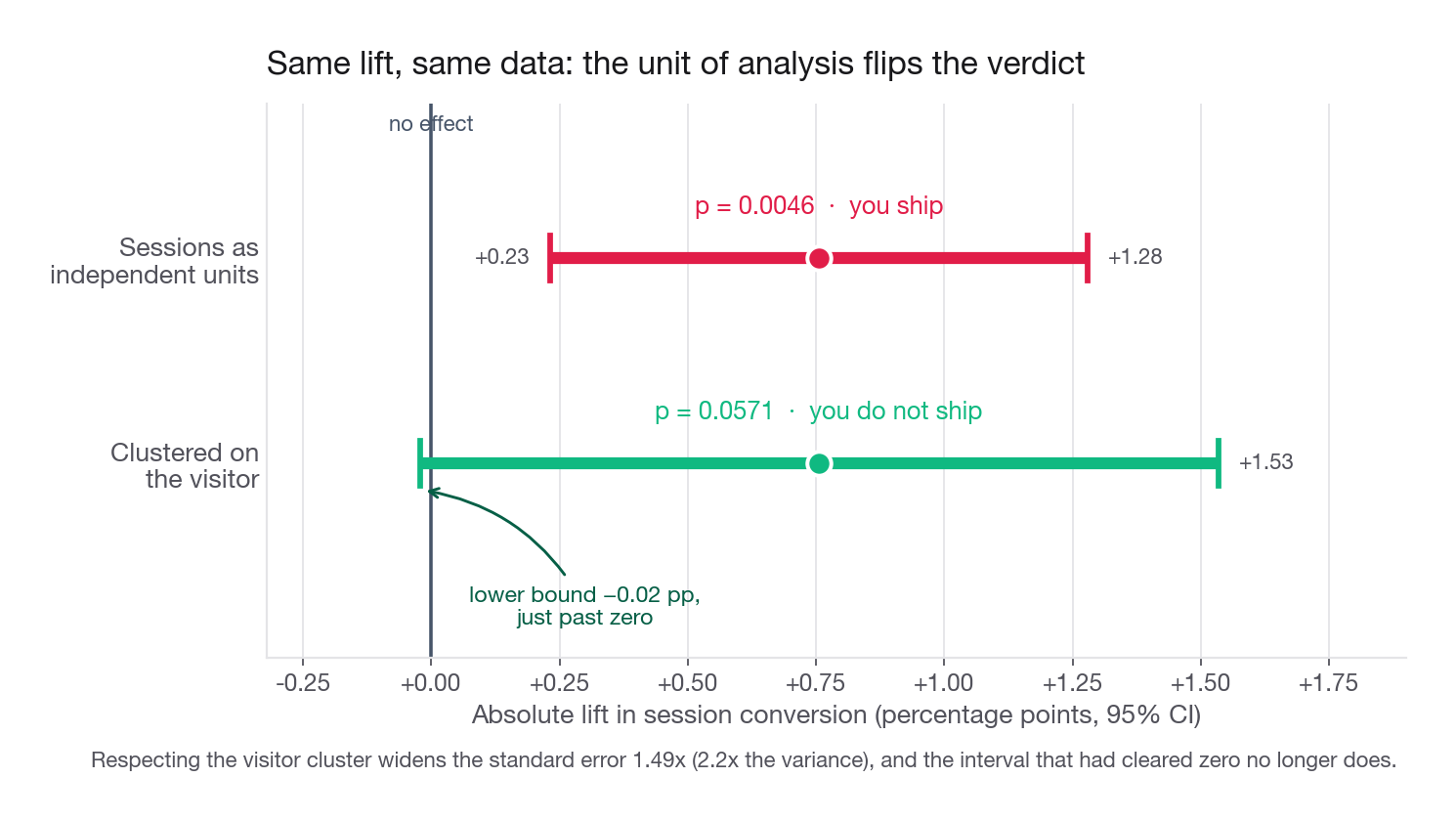
naive session diff=0.00756 se=0.00267 p=0.0046
visitor cluster diff=0.00756 se=0.00397 p=0.0571Identical point estimate. Standard error 1.49 times larger once you respect the clustering, which is a variance ratio of 2.2. The naive analysis reports p equal to 0.0046 and you ship. The correct one reports p equal to 0.057 and you do not. Same data, opposite decision, and the only difference is whether you counted sessions or visitors as the independent unit.
Three ways to fix it.
Aggregate to the randomization unit. One number per visitor, then a two-sample test on visitors. Simple and always defensible, slightly wasteful because it weights a 1-session visitor like a 12-session one.
Delta method on the ratio. Keep the ratio-of-sums metric and correct its variance for clustering, as above. This is what most in-house experiment platforms do.
Cluster-robust standard errors. Regress the outcome on the treatment indicator, clustering errors on visitor. Equivalent in spirit, convenient when you also want covariate adjustment.
Interview tip: When you are handed a session-level or event-level metric, ask "what was randomized?" out loud. If the answer is anything coarser than the metric's denominator, say you will cluster on the randomization unit before you say anything else about the result.
Choosing the assignment unit
The bottom two rows are where the interesting interview questions live, and they get a full lesson later in the section. For now the rule of thumb is: randomize on the coarsest unit that removes contamination, and no coarser, because every step coarser costs you effective sample size.
The primary metric and its guardrails
Exactly one primary metric
Pick one. Not two, not "conversion and revenue." The reason is not statistical purity: two primary metrics with no stated priority means that when they disagree, whoever argues hardest wins the meeting. You wrote the decision statement to prevent exactly that. A usable primary metric clears four bars.
It is computable. Numerator, denominator, population, window. "Booking rate" is ambiguous. "Share of assigned visitors with at least one completed booking within 7 days of first exposure" is not.
It is sensitive to the change. If the change touches room selection and the primary metric is 90-day retention, you picked a number the treatment can barely move and noise easily swamps. The primary metric should sit as close to the mechanism as the decision allows.
It cannot move for the wrong reason. Bookings per visitor rises if you make cancelling harder. Pages per session rises if you break navigation. Ask what the laziest way to move the number would be, and if the treatment could take that route, add a guardrail that catches it.
It matches the decision. If the decision is a funding decision about revenue, a pure engagement metric will not settle it, however clean.
For Bellhop the primary metric is booking rate per assigned visitor: the share of visitors assigned to an arm who complete at least one booking within 7 days of assignment. Assigned, not exposed, which matters and is picked apart in the randomization lesson.
Guardrails
A guardrail is a metric you are not trying to move but are not willing to damage. Three or five of them, each with a direction and a numeric stop rule written before launch. Without the stop rule they are decoration.
| Guardrail type | What it protects | Bellhop example | Stop rule agreed in advance |
|---|---|---|---|
| Counter-metric | The obvious way to game the primary | Net revenue per assigned visitor, booking value with cancelled bookings removed | Kill if the lift is below -1 percent relative and the interval excludes zero |
| Quality | The value of the thing being produced | Cancellation rate among bookings | Escalate if it rises by more than 5 percent relative |
| Health | The system itself | p95 search latency | Halt the test if it rises by more than 80 ms |
| Trust | The relationship, not this session | Support contacts per 1,000 visitors | Escalate on any increase with p below 0.01 |
| Ecosystem | The other side of the market | Share of listings receiving an impression | Escalate if it falls by more than 2 points |
Guardrails are asymmetric. You are not testing whether they improved, only whether they got worse by enough to matter, which is why several are one-sided by nature.
Interview tip: Name a guardrail that the interviewer did not expect. For a booking flow, support contacts per 1,000 visitors is a good one, because it catches confusion that conversion metrics are blind to.
One-sided versus two-sided
Candidates get asked this constantly and answer it badly, usually by reciting that one-sided has more power. That is true and it is not the point.
The real question is whether a result in the unexpected direction changes what you do. If a large drop would make you kill the feature, investigate, or write a postmortem, that outcome is a distinct decision and you need a two-sided test. If a decline leads to exactly the same action as a null result, one-sided is coherent. In practice two-sided on the primary metric is the default nearly everywhere, because a significant regression is useful information and because picking one-sided once you know the direction is dishonest.
| Two-sided | One-sided | |
|---|---|---|
| Question answered | Did the metric change at all | Did the metric improve by more than nothing |
| Power at fixed n | Lower | Higher, roughly the power of a two-sided test at twice the alpha |
| Detects a regression | Yes, with the same rigour | No, a large drop returns a p-value near 1 |
| Bellhop primary metric, observed | p equal to 0.00045 | p equal to 0.00022 |
| When it is defensible | Default for any primary metric | Guardrails, where you only care about the harmful direction, and it is declared before launch |
| How it goes wrong | Slightly conservative | Chosen after seeing the data, which is p-hacking with extra steps |
The Bellhop row is deliberately boring: at z equal to 3.51, the choice does not affect the decision at all. That is usually the case. The choice matters exactly in the region where a result is marginal, which is exactly the region where you must not be seen to have chosen it opportunistically.
Interview tip: Answer with "two-sided on the primary metric, because a significant regression changes what I do; one-sided on guardrails, because there I only care about the bad direction." That is the full answer in one sentence.
The comparison itself
Now the arithmetic. The test is the least interesting part of the lesson and it takes about ten lines.
Everything below runs on a synthetic Bellhop result table generated deterministically by this block. One row is one assigned visitor over the 7-day attribution window.
import numpy as np
import pandas as pd

SEED = 41077
rng = np.random.default_rng(SEED)

N = 361_400
arm = rng.choice(["control", "treatment"], N, p=[0.5, 0.5])
device = rng.choice(["ios", "android", "desktop"], N, p=[0.31, 0.34, 0.35])
market = rng.choice(["NA", "EMEA", "APAC"], N, p=[0.44, 0.36, 0.20])
member = rng.random(N) < 0.27
is_t = arm == "treatment"

base = 0.049 + 0.020 * member + np.select(
    [device == "desktop", device == "ios"], [0.011, 0.004], 0.0)
p_book = np.clip(base + np.where(is_t, 0.0022, 0.0), 0.001, 0.4)
booked = rng.random(N) < p_book

nights = np.where(booked, rng.integers(1, 6, N), 0)
adr = rng.normal(np.where(is_t, 162.0, 168.0), 34.0).clip(45.0, 600.0)
cancelled = booked & (rng.random(N) < np.where(is_t, 0.081, 0.104))

bellhop = pd.DataFrame({
    "visitor_id": np.arange(1, N + 1),
    "arm": arm, "device": device, "market": market,
    "is_member": member.astype(int),
    "booked": booked.astype(int),
    "room_nights": nights,
    "booking_value": np.round(nights * adr, 2),
    "cancelled": cancelled.astype(int),
})
print(bellhop.groupby("arm")["booked"].agg(["size", "mean"]).round(5))
size mean
arm
control 180720 0.05941
treatment 180680 0.06220One thing to check before any test. The arms are 180,720 and 180,680, a split of 50.006 to 49.994 percent, which is fine. A split improbably far from 50/50 is a sample ratio mismatch, it invalidates everything downstream, and it is the first thing to look at on a real result. The randomization lesson covers it properly.
The comparison, three equivalent ways
The metric is binary, so each observation is a Bernoulli draw. People argue about two-proportion z, chi-squared, or Welch's t-test on the 0/1 column. At these sample sizes they agree to three decimals, and the t-test is the one you will see most often because it generalizes to continuous metrics with no code change.
from scipy import stats

g = bellhop.groupby("arm")["booked"]
n, p = g.size(), g.mean()
p_c, p_t = p["control"], p["treatment"]
n_c, n_t = n["control"], n["treatment"]

diff = p_t - p_c
se = np.sqrt(p_c * (1 - p_c) / n_c + p_t * (1 - p_t) / n_t)
z = diff / se
lo, hi = diff - 1.96 * se, diff + 1.96 * se

print(f"control {p_c:.5f}  treatment {p_t:.5f}")
print(f"absolute lift {diff*100:.4f} pp   se {se*100:.4f} pp   z {z:.3f}")
print(f"two-sided p {2*stats.norm.sf(abs(z)):.5f}")
print(f"relative lift {100*diff/p_c:.2f}%  CI [{100*lo/p_c:.2f}%, {100*hi/p_c:.2f}%]")
control 0.05941 treatment 0.06220
absolute lift 0.2792 pp se 0.0795 pp z 3.511
two-sided p 0.00045
relative lift 4.70% CI [2.08%, 7.32%]Welch's t-test on the same column returns t equal to 3.511 and the same p-value, since with 180,000 rows per arm the t distribution is indistinguishable from the normal. Why Welch rather than pooled variance: for a Bernoulli the variance is a function of the mean, so two arms with different means have different variances, and the unequal-variance version is the honest default at no cost.
Report the interval, not the p-value
The p-value answers a question nobody asked: how surprising is this data if the change did nothing. The decision needs a different question: what range of true effects is compatible with what we saw.
Booking rate rose 4.70 percent relative, interval 2.08 to 7.32. The decision statement promised to ship at 3 percent or better. The point estimate clears the bar; the interval's lower end does not. Honest summary: the effect is almost certainly positive, most likely near 4.7 percent, and the data cannot rule out a true effect of 2.1 percent, which is below the threshold you agreed to.
A p-value of 0.00045 hides that entire sentence. This is why "significant, therefore ship" is the answer of a junior candidate, and why the sizing lesson insists you choose the minimum detectable effect from business value before you start.
Absolute or relative
Report both, and know which one the decision needs.
Absolute lift, 0.2792 percentage points, is what you multiply by traffic to get incremental bookings: at Bellhop's roughly 4.1 million monthly visitors, about 11,400 extra bookings a month. Relative lift, 4.70 percent, is what you compare against other experiments and against the minimum detectable effect, because it is scale-free. The trap is that relative lift on a small base looks enormous and means little. A guardrail moving from 0.02 to 0.03 percent is a 50 percent increase and 1 extra event per 10,000 visitors. Show both, especially for guardrails.
From a result to a launch recommendation
Now the whole read. The primary metric plus every guardrail, each with a relative lift and an interval.
def compare(frame, col):
    t = frame.loc[frame.arm == "treatment", col]
    c = frame.loc[frame.arm == "control", col]
    d = t.mean() - c.mean()
    se = np.sqrt(t.var(ddof=1) / len(t) + c.var(ddof=1) / len(c))
    return {"metric": col, "control": c.mean(), "treatment": t.mean(),
            "rel_%": 100 * d / c.mean(),
            "lo_%": 100 * (d - 1.96 * se) / c.mean(),
            "hi_%": 100 * (d + 1.96 * se) / c.mean(),
            "p": 2 * stats.norm.sf(abs(d / se))}

bellhop["net_revenue"] = bellhop["booking_value"] * (1 - bellhop["cancelled"])
rows = [compare(bellhop, c) for c in
        ["booked", "booking_value", "net_revenue", "cancelled"]]
booked_only = bellhop[bellhop.booked == 1]
rows.append({**compare(booked_only, "booking_value"), "metric": "value_per_booking"})
rows.append({**compare(booked_only, "cancelled"), "metric": "cancel_rate_of_bookings"})
print(pd.DataFrame(rows).round(4).to_string(index=False))
metric control treatment rel_% lo_% hi_% p
booked 0.0594 0.0622 4.6986 2.0758 7.3214 0.0004
booking_value 29.7337 29.9470 0.7173 -2.2069 3.6415 0.6307
net_revenue 26.6359 27.5698 3.5062 0.3880 6.6244 0.0275
cancelled 0.0062 0.0050 -19.1234 -26.9851 -11.2617 0.0000
value_per_booking 500.4639 481.4331 -3.8026 -5.1628 -2.4425 0.0000
cancel_rate_of_bookings 0.1041 0.0804 -22.7529 -30.1087 -15.3972 0.0000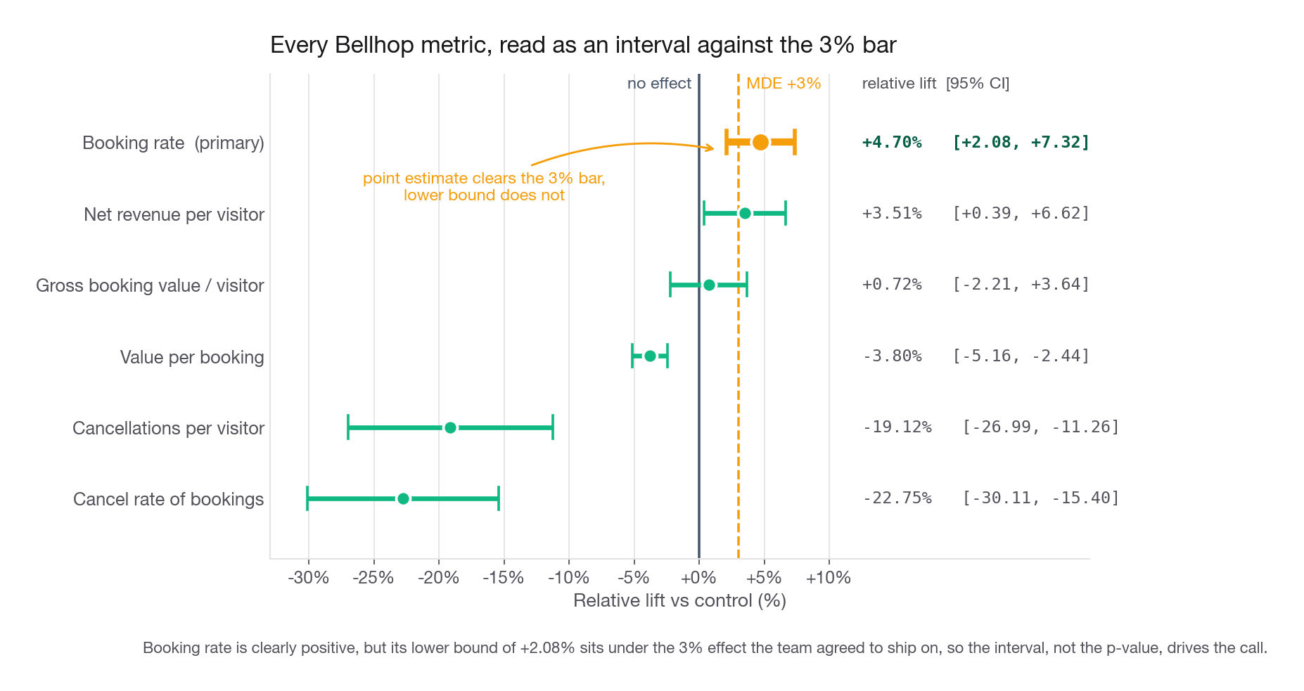
This table is a genuinely interesting result and a good thing to talk through out loud.
Two rows need a warning label first. value_per_booking and cancel_rate_of_bookings condition on booked == 1, and booking is itself an outcome the treatment moved by 4.70 percent, so neither is protected by randomization any more: the treatment arm's booker pool contains marginal bookers who would not have booked under control. How much that matters is boundable, and the bound is the thing to say out loud. Marginal bookers are 4.5 percent of the treatment booker pool, so a mix shift can move a per-booking metric by at most 4.5 percent times the marginal-to-always gap. For value per booking that ceiling is wide open: a marginal booking need only be 85 percent cheaper than average to produce the whole -3.80 percent, and the cheapest booking this data allows, one night at the 45 dollar floor, is 91 percent below the control mean. For cancellation rate it binds hard: even if marginal bookers never cancelled, composition covers only 4.5 points of the 22.8 percent fall. Read the first row as a diagnostic and the second as evidence.
The primary metric moved. Booking rate is up 4.70 percent relative, interval clear of zero.
Bookings got smaller, and this row cannot tell you why. Value per booking fell 3.80 percent, interval -5.16 to -2.44. It is consistent with the predicted mechanism, people choosing a cheaper room once the total is visible, and because the hypothesis anticipated it nobody is panicking. But the identical number appears if nobody traded down and the change merely recruited cheaper bookers. What randomization does support is the aggregate version: booking rate up 4.70 percent against gross booking value per assigned visitor up only 0.72 percent, so the average booking is smaller either way. Separating the two stories needs a split on a pre-assignment segment, or the 90-day repeat-booking readout.
The two effects nearly cancel on gross booking value. Gross booking value per assigned visitor is up 0.72 percent, interval -2.21 to +3.64, p equal to 0.63. Gross sits in the readout as a diagnostic, not the guardrail, there to make the offset visible: more bookings at a lower average value landing on top of each other. Not a win, not a loss, just a number that cannot see the difference.
Cancellations fell hard. Cancellation rate among bookings dropped from 10.41 percent to 8.04 percent, a 22.8 percent relative fall. Fewer people are booking and then discovering the real price.
The pre-registered revenue guardrail ends up positive. Net revenue per assigned visitor, the definition written into the design document before launch, is up 3.51 percent with an interval from 0.39 to 6.62. Note how thin that lower bound is: it clears zero, but only just, so this is directional corroboration, not a second precise win.
The four outcome quadrants
Every result lands in one of four boxes, defined by whether the interval excludes zero and whether it clears the effect you said you needed. Learn them.
| Interval excludes zero | Interval clears the MDE | What it means | What to recommend |
|---|---|---|---|
| Yes | Yes | Clear win at or above the size you needed | Ship, and state the expected annualized impact |
| Yes | No, lower bound below the MDE | Real effect, possibly smaller than the bar you set | Ship if reversal cost is low, otherwise extend to tighten the interval |
| No | Interval fully inside plus or minus the MDE | Precisely estimated null, a genuine result | Do not ship, and say the change is ruled out at the size that would have mattered |
| No | Interval wider than the MDE | Underpowered, you learned nothing | Do not ship and do not claim it failed; either extend or admit it was not worth testing |
The third row is the one candidates never volunteer and it is worth points. A tight null is a real finding: you ruled out an effect large enough to care about, which is a service to everyone who would have kept proposing it. The fourth row is a design failure a power calculation should have prevented. Bellhop's primary metric is row two.
The recommendation, out loud
Here is a weak version.
"The test won, p equals 0.0004, conversion is up 4.7 percent. I would ship it."
That is not wrong and it is not enough. Here is the stronger version.
"Ship it, with one caveat. Booking rate is up 4.70 percent relative, interval 2.08 to 7.32, so the effect is real. But we agreed to ship at 3 percent and the lower bound is 2.08, so a true effect below our bar is compatible with the data. The reason I still recommend shipping is the guardrail picture: cancellations among bookings fell 22.8 percent and net revenue per visitor is up 3.51 percent with an interval clear of zero. On the mechanism I want to be careful. Value per booking is down 3.80 percent, which is consistent with people trading down once they can see the total, but I would not state that as fact: it conditions on booking, and a change that recruits cheaper bookers produces the same figure. What is safe either way is that booking rate rose 4.70 percent while gross booking value per visitor rose only 0.72 percent, so the average booking is smaller. To separate the two I would split on a pre-assignment segment, never on anything measured after assignment. As pre-registered, the revenue guardrail is net of cancellations; gross is in the readout only to make the offset visible. If someone wants the interval tightened before rolling to 100 percent, two more weeks at the current allocation would roughly halve it, and I would rather spend that time on the 90-day repeat-booking readout, because the trade-down effect is the thing that could look different over a longer horizon."
That answer states the recommendation first, admits the weakness in the primary result, uses the guardrails as corroboration rather than decoration, ties the pattern back to the stated mechanism, and names the follow-up.
Interview tip: Always lead with the recommendation, then the caveat. Candidates who narrate the analysis for two minutes and arrive at a verdict at the end read as uncertain even when the analysis is perfect.
Common traps
Designing the metric before the decision. You get a beautifully specified number nobody will act on. Fix: write the decision statement first, with the no-action branch spelled out.
Two primary metrics. When they disagree, the decision is settled by seniority instead of evidence. Fix: one primary, everything else a guardrail with a stop rule.
Randomizing by visitor and testing by session. The most common quiet error in this whole topic. It shrinks the standard error by 1.5 times or more and flips marginal results to significant. Fix: aggregate to the randomization unit, or use the delta method or cluster-robust errors.
Treating significance as the ship rule. With 4 million monthly visitors you can detect effects far too small to fund. Fix: state a minimum detectable effect from business value up front and compare the interval against it, not the p-value against 0.05.
Choosing one-sided after seeing the direction. It nearly doubles your alpha in secret. Fix: declare sidedness in the pre-registration; two-sided on the primary metric by default.
Reporting a relative lift with no absolute number. A guardrail going from 0.02 to 0.03 percent is a 50 percent increase and almost nothing. Fix: show both, always.
Redefining the metric after seeing the result. Gross and net revenue disagree here, 0.72 percent with p equal to 0.63 against 3.51 percent with p equal to 0.028, and picking whichever supports your recommendation is post hoc metric selection in a clean shirt. It is the two-primary-metrics failure, one step later. Fix: write the exact numerator and denominator into the pre-registration, and label any second definition a diagnostic before anyone has seen its number.
Slicing until something is significant. The Bellhop generator adds the same 0.22 percentage points to every treatment row regardless of device, so all three device slices estimate one true effect: about 3.8 percent relative, against iOS's true control rate of 5.84 percent. Yet Android reads +2.07 percent with p equal to 0.38, desktop +2.04 percent with p equal to 0.34, and iOS +11.13 percent with p equal to 0.0000095. Be precise about what went wrong, because the obvious reading is wrong. This is not a false positive, and correcting for multiple comparisons does not touch it: Bonferroni over three slices sets the threshold at 0.0167, that p-value clears it by three orders of magnitude, and it would take roughly 5,250 comparisons to stop being significant at 0.05. There is no iOS-specific effect. The damage is that +11.13 percent is nearly three times the true 3.8 percent: the slice you noticed is the slice that got lucky, so any segment singled out for being significant overstates its own effect. This draw is also extreme: across 400 seeds of the same generator the median smallest device-slice p is about 0.015, and only 2.5 percent produce any slice below 0.00001. Fix: name segments before launch, quote the pre-registered overall effect as the estimate, and treat an unplanned slice's magnitude as an upper bound, not a finding.
Confusing assignment with exposure. Counting only visitors who reached the changed screen sounds sensible and quietly breaks randomization, because reaching it is itself affected by the treatment. Fix: analyse everyone assigned, and treat dilution as a separate design choice.
Forgetting the reversal cost. Testing a copy change that could have shipped in an hour burns traffic and calendar a higher-stakes test needed. Fix: ask what it costs to undo, and let that set how much evidence you buy.
Declaring a null result a failure. A tight interval around zero is real information. Fix: report the interval and say plainly either that an effect large enough to matter is ruled out, or that the test was underpowered and nothing was learned. Only one of those is an excuse.
Quick self-check
Answer these out loud, in full sentences. If you stumble, that is the section to reread.
A product manager asks you to test a new listing card layout. Before you mention any metric, what three questions do you ask, and what does each answer change about your design?
You randomize by account and the metric is messages per conversation. Are the units the same? If not, what goes wrong in a naive two-sample test, roughly how large is the error, and what are two fixes?
Your primary metric is up 1.2 percent relative with a 95 percent interval from -0.4 percent to 2.8 percent, and you pre-registered a minimum detectable effect of 2 percent. Which of the four outcome quadrants is this, and what exactly do you recommend?
Name three guardrails for a test that adds one-click reordering to a food delivery app, and give each one a numeric stop rule. Explain what specific bad outcome each guardrail is there to catch.
When is a one-sided test defensible, and what is the one condition that makes it indefensible regardless of the metric?
Bookings are up 4.7 percent and gross revenue per visitor is flat. Give the two-sentence explanation of how both can be true, say why the only defensible headline definition is whichever one you pre-registered, and name the row in the results table you would refuse to call a causal estimate.
The next lesson turns "minimum detectable effect" into a calculation, works out how long the Bellhop test had to run, and shows why halving a confidence interval costs four times the data.