5.3 Multiple Tests, Sample Size Traps, and When Not to Test
Find the core decision, design, or behavior signal.
Turn the lesson into a concise response blueprint.
Name the trap you would avoid in a real interview.
Use these checkpoints as your reading path before diving into the full lesson.
- 1Why this matters in interviews
- 2The three questions hiding inside "we r...
- 3The program you will reason about
- 4Question one: do concurrent tests inter...
- 5Why independent randomization saves you
Almost every experimentation question you get in a senior loop is about one test. This lesson is about the other situation, the one that describes your actual job: a company running two hundred tests a quarter, a homepage team running thirty variants in parallel, a product manager who wants to call a winner on Tuesday, a brand-new recommender that has learned nothing yet, and a rebrand nobody can randomize at all. The decision here is not "did this variant win". It is "how much of what we shipped last quarter was real, and what do we do about the changes we cannot test".
Why this matters in interviews
The classic prompt is short. "We ran thirty versions of our homepage. One beat control with a p-value of 0.04. Ship it?" A junior candidate says no and recites Bonferroni. That is correct and worth about four points out of ten, because it stops where the interesting part starts.
The strong version does four more things. It quantifies how likely a spurious winner was in the first place. It separates controlling the family-wise error rate from controlling the false discovery rate, and says which one a test program actually wants. It notices that a p-value of 0.04 is the weakest possible member of the winners club. And it ends with a policy rather than a verdict, because the interviewer wants to know whether you can run an experimentation program, not whether you memorised a correction factor.
Section 4.4 handled multiplicity inside one experiment: many metrics, one test. This lesson handles multiplicity across a program: many tests, one quarter. They look similar on a slide and have different fixes.
Our fictional company throughout is Halcyon, a marketplace for used and out-of-print books, roughly 3.1 million monthly buyers, web plus two apps. The primary experiment metric on most surfaces is item-page purchase rate, currently 4.12 percent.
The three questions hiding inside "we run a lot of tests"
When an interviewer says "we run a lot of tests", they may be asking any of three different things. Answer the wrong one and you sound like you are dodging.
| The prompt sounds like | The real question | The tool |
|---|---|---|
| "We have thirty tests live on the homepage at once" | Do concurrent experiments contaminate each other? | Randomization layers, and an interaction check |
| "One of thirty beat control at 0.04" | How many of my declared winners are noise? | False discovery rate over the program |
| "We only get 9,000 visitors a week on that surface" | This test cannot answer the question. What instead? | Variance reduction, triggering, pooling, or judgment |
Say which one you are answering before you answer it. Two sentences of framing at the top of a case buys more credit than any single technical point later.
Interview tip: Open with "there are three separate problems bundled into that sentence, and I want to take them in order", then name them. It reframes a trivia question as a systems question.
The program you will reason about
Every number below comes from one synthetic quarter of Halcyon experiments. This block builds it deterministically from numpy and pandas only. Each row is one test: traffic, whether the change genuinely moved the purchase rate, the observed lift, and the resulting p-value.
import math
import numpy as np
import pandas as pd

SEED = 20260826
rng = np.random.default_rng(SEED)

N_TESTS = 240          # experiments completed in one quarter at Halcyon
BASE = 0.0412          # item-page purchase rate
PRIOR_REAL = 0.22      # share of proposals that genuinely move the metric

surface = rng.choice(
    ["item_page", "search", "cart", "lifecycle_email", "app_home"],
    size=N_TESTS, p=[0.30, 0.22, 0.18, 0.15, 0.15])
week = rng.integers(1, 14, size=N_TESTS)
n_per_arm = rng.integers(30_000, 220_000, size=N_TESTS)

is_real = rng.random(N_TESTS) < PRIOR_REAL
true_lift = np.where(is_real, rng.normal(0.0011, 0.0013, N_TESTS), 0.0)
se = np.sqrt(2 * BASE * (1 - BASE) / n_per_arm)
obs_lift = true_lift + rng.normal(0.0, se)
z = obs_lift / se
p_value = np.vectorize(math.erfc)(np.abs(z) / math.sqrt(2))

program = pd.DataFrame({
    "test_id": [f"HX-{i:03d}" for i in range(1, N_TESTS + 1)],
    "surface": surface, "week": week, "n_per_arm": n_per_arm,
    "is_real": is_real, "true_lift": true_lift,
    "obs_lift": obs_lift, "se": se, "p_value": p_value,
})
program["ship_naive"] = (program.p_value < 0.05) & (program.obs_lift > 0)
print(len(program), int(program.is_real.sum()), int(program.ship_naive.sum()))
240 47 21Read those three numbers carefully. Of 240 completed tests, 47 changes genuinely moved the purchase rate. Under the house rule of "significant and positive, ship it", 21 shipped. The overlap is the interesting part.
Typical standard error here is about 0.09 percentage points on a 4.12 percent base, so a test at median traffic reliably detects a lift of roughly 0.25 points, a relative 6 percent. Most real effects at Halcyon are smaller than that, which is the ordinary condition of a mature product rather than a flaw in the simulation.
Question one: do concurrent tests interfere with each other?
The instinctive worry is that thirty simultaneous homepage tests must be scrambling each other's results. Usually they are not.
Why independent randomization saves you
If each experiment assigns users independently, the other twenty-nine tests distribute themselves evenly across any given test's two arms. A user in HX-041's treatment is exactly as likely to be in HX-112's treatment as a user in HX-041's control. Whatever HX-112 does to the purchase rate, it does equally to both of HX-041's arms, so it cancels in the difference.
Formally: concurrent experiments are a nuisance factor balanced by randomization, so your estimate stays unbiased while residual variance rises, costing a little power.
The layer system
Real platforms make that guarantee explicit. Traffic is divided into layers. Within a layer, experiments are mutually exclusive, so two variants that both rewrite the buy box can never collide on one user. Across layers, assignment is independent, usually by hashing the user id with a per-layer salt so the buckets are uncorrelated. Halcyon runs a buy-box layer, a search-ranking layer, a lifecycle-messaging layer, and a catch-all. If you cannot describe this mechanism, it shows.
| Design | What it guarantees | What it costs | Use it when |
|---|---|---|---|
| Independent overlap across layers | Unbiased estimates everywhere, all traffic reusable | Slightly wider intervals, undetected interactions | Default, for most tests |
| Mutual exclusion inside one layer | No user sees two conflicting versions of a surface | Traffic is divided, so each test runs longer | Two tests edit the same element, or the combination is broken |
| Deliberate factorial | The interaction is estimated, not assumed away | Roughly four times the traffic per cell | You genuinely expect the changes to reinforce or cancel |
Checking for an interaction you did not predict
Overlap hurts when two changes interact: a price badge and a new sort order might each help alone but fight together, or a discount banner might swallow a free-shipping badge because a user responds to only one incentive. Each marginal estimate stays unbiased, but it is now an average over the other test's arms, which is not the number you get after both ship. You check by building the 2 by 2.
rng2 = np.random.default_rng(515)
N = 400_000
a = rng2.integers(0, 2, N)          # HX-041: new item-page sort order
b = rng2.integers(0, 2, N)          # HX-112: price-history badge
prob = BASE + 0.0018 * a + 0.0012 * b - 0.0009 * a * b
bought = rng2.random(N) < prob

cells = (pd.DataFrame({"sort_v2": a, "badge": b, "bought": bought})
         .groupby(["sort_v2", "badge"]).bought.agg(["mean", "size"]))
m, n_cell = cells["mean"].values, cells["size"].values
interaction = (m[3] - m[2]) - (m[1] - m[0])
se_cell = np.sqrt(BASE * (1 - BASE) / n_cell)
se_int = np.sqrt((se_cell ** 2).sum())
print((cells["mean"] * 100).round(3).to_string())
print(f"interaction {interaction*100:+.3f} pts, se {se_int*100:.3f}, "
      f"z {interaction/se_int:.2f}")
sort_v2 badge
0 0 4.090
1 4.233
1 0 4.326
1 4.443
interaction -0.026 pts, se 0.126, z -0.21The truth in this simulation is an interaction of negative 0.09 points, and the check found nothing. That is the point, not a failure.
With four cells of 100,000 users, a main effect carries a standard error of about 0.063 points and the interaction 0.126 points, exactly twice as wide, because a difference of differences takes all four cell variances at full weight. Twice the standard error means four times the sample for equal precision. Interactions are also usually smaller than main effects, often half the size, so detecting one takes roughly sixteen times the traffic. A routine interaction check is underpowered by design, and its null result is close to uninformative.
The honest policy is therefore not "test for interactions". It is: force exclusivity when product logic says two changes fight, overlap otherwise, and accept the residual risk explicitly.
Interview tip: Say "the interaction term carries twice the standard error of a main effect, so a routine check needs sixteen times the traffic to catch something half the size, which is why we gate on product judgment instead."
Question two: thirty variants, one winner at p equals 0.04
The number to say out loud
Suppose all thirty variants are duds. Each still has a 5 percent chance of a significant p-value by luck, and half of those land the wrong way, so each dud has a 2.5 percent chance of clearing the bar in the winning direction. That 0.025, the rate the ship-on-significant-and-positive rule actually exposes you to, is the same one the Bayes calculation later in this lesson uses. The chance at least one dud wins is 1 minus 0.975 to the thirtieth, which is 53 percent. You expected about three quarters of a spurious winner and got one. Halcyon's quarter says the same thing empirically: of its 193 tests where nothing was really there, 8 fired in one direction or the other but only 4 cleared the ship rule, a 2.1 percent false-winner rate rather than 5. The result is unsurprising under the null, and unsurprising under the null is the definition of no evidence. Say that arithmetic aloud. It takes thirty seconds and converts a memorised rule into demonstrated understanding.
Bonferroni, and what it costs
The textbook fix divides the threshold by the number of tests: 0.05 over 30 is 0.00167, so 0.04 is twenty-four times too large. You do not ship.
Bonferroni controls the family-wise error rate, the chance of making even one false claim. That is right when a single false claim is catastrophic: a drug approval, a safety recall, a legal filing. It is expensive when the cost of a false claim is a homepage tweak that does nothing.
Watch what it does to Halcyon's quarter. Across all 240 tests the threshold becomes 0.000208. Two tests survive, both genuinely real, and 45 of the 47 real effects are discarded, including 33 of the 35 that were genuine improvements. The other 12 real effects were genuine harms, and no rule here ships those anyway, since all three require a positive observed lift, so they sit outside the trade. That is a program that ships almost nothing and calls it rigour.
Why family-wise control is the wrong instrument here
The mismatch is about which error you are pricing. Across a quarter you do not care whether you made zero mistakes. You care what share of your shipped wins were mistakes, because that share decides whether your roadmap forecast is honest. Shipping 16 wins of which 1 is fake beats shipping 2 wins of which 0 are fake, even though the second is safer by the family-wise standard. Controlling the false discovery rate targets exactly that share.
The Benjamini-Hochberg procedure is four lines. Sort p-values ascending, compare the i-th against q times i over m, find the largest i that passes, reject everything up to it.
def benjamini_hochberg(p, q=0.10):
    order = np.argsort(p)
    m = len(p)
    thresh = q * (np.arange(1, m + 1)) / m
    passing = np.nonzero(p[order] <= thresh)[0]
    keep = np.zeros(m, dtype=bool)
    if passing.size:
        keep[order[: passing.max() + 1]] = True
    return keep

positive = program[program.obs_lift > 0].copy()
positive["ship_bh"] = benjamini_hochberg(positive.p_value.values, q=0.10)
sel = positive[positive.ship_bh]
print(f"candidates {len(positive)}  selected {len(sel)}  "
      f"actually real {int(sel.is_real.sum())}  "
      f"realised FDR {1 - sel.is_real.mean():.1%}")
candidates 121 selected 16 actually real 15 realised FDR 6.2%| Rule | Threshold | Shipped | False ships | Real effects missed | Realised FDR |
|---|---|---|---|---|---|
| Uncorrected, p below 0.05 and positive | 0.05 | 21 | 4 | 30 | 19.0 percent |
| Bonferroni across the quarter | 0.000208 | 2 | 0 | 45 | 0 percent |
| Benjamini-Hochberg at q equal to 0.10 | adaptive | 16 | 1 | 32 | 6.2 percent |
Bonferroni bought four avoided mistakes at a price of fifteen forgone real improvements. Count that carefully: 21 ships drop to 2, but 4 of the 19 it gives up are the fakes it is being credited with catching, so the price is 15, not 19. Benjamini-Hochberg bought three of those four for a price of two. On a product roadmap that trade is not close.
Interview tip: Do not stop at "I would use Bonferroni". Say "Bonferroni controls the chance of any false claim, which is the wrong target for a roadmap. I would control the false discovery rate, and here is what that buys."
The number nobody computes: how many shipped wins are real
Here is the move separating a strong candidate from a very strong one. Reverse the conditional. A p-value gives the probability of your data given no effect. Your VP wants the probability of an effect given your data.
For a program that is one line of Bayes. Let r be the share of proposals that genuinely work and let power be the chance a real effect clears your bar. A two-sided test at 0.05 that you only ship on when the lift is positive has an effective one-sided false-positive rate of 0.025.
def prob_real_given_win(prior, power, alpha=0.025):
    return prior * power / (prior * power + (1 - prior) * alpha)

for prior in (0.10, 0.20, 0.35, 0.50):
    row = [f"{prob_real_given_win(prior, pw)*100:.0f}%"
           for pw in (0.20, 0.40, 0.60, 0.80)]
    print(f"prior {prior:>5.2f}  " + "  ".join(f"{v:>4}" for v in row))
prior 0.10 47% 64% 73% 78%
prior 0.20 67% 80% 86% 89%
prior 0.35 81% 90% 93% 95%
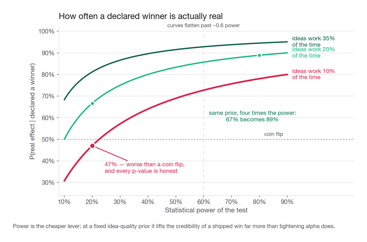
prior 0.50 89% 94% 96% 97%Read the top-left cell. A team whose ideas work one time in ten, running tests at 20 percent power, ships winners that are real less than half the time. Nothing about their process is wrong and every p-value is honest. The program still produces coin flips, and will until idea quality or power goes up.
Now read across a row. Moving from 20 to 80 percent power at a fixed prior of 0.20 takes you from 67 percent to 89 percent. Tightening alpha from 0.05 to 0.01 at 20 percent power gets you to 91 percent, but holding power there costs about 2.4 times the sample per test, so on a fixed traffic budget you run fewer than half as many tests and find roughly 70 percent fewer wins. Power is the cheaper lever, and almost nobody says so.
A p-value of 0.04 is the weakest member of the winners club
That 80 percent figure averages over all winners, including those that cleared the bar by a mile. A result sitting at 0.04 is the marginal one. Bin winners by evidence strength using a large replicate of the same generative model.
Z = {"p05": 1.959964, "p03": 2.170090, "p01": 2.575829}
rng3 = np.random.default_rng(3001)
M = 400_000
real_m = rng3.random(M) < PRIOR_REAL
lift_m = np.where(real_m, rng3.normal(0.0011, 0.0013, M), 0.0)
se_m = np.sqrt(2 * BASE * (1 - BASE) / rng3.integers(30_000, 220_000, M))
z_m = (lift_m + rng3.normal(0, se_m)) / se_m

bands = [("0.03 to 0.05", Z["p05"], Z["p03"]),
         ("0.01 to 0.03", Z["p03"], Z["p01"]),
         ("below 0.01", Z["p01"], np.inf)]
for label, lo, hi in bands:
    mask = (z_m >= lo) & (z_m < hi)
    print(f"p {label:<13} n={mask.sum():>6}  really moved the metric "
          f"{real_m[mask].mean():5.1%}")
p 0.03 to 0.05 n= 6672 really moved the metric 53.6%
p 0.01 to 0.03 n= 9233 really moved the metric 67.0%
p below 0.01 n= 23761 really moved the metric 93.3%A winner between 0.03 and 0.05 is real 54 percent of the time here. A winner below 0.01 is real 93 percent of the time. Treating both as "significant" throws away most of the information you paid for.
So the full answer has two independent reasons. First, with thirty tests you expected about three quarters of a spurious winner and got one. Second, even with a single pre-registered test, 0.04 in a program with this much power would be real about half the time. Multiplicity made a weak signal weaker; it did not create the weakness.
Interview tip: Add "and separately from multiplicity, a p-value right at the boundary is the least convincing kind of win, because in a program with our power roughly half the results in that band are noise."
The same error in different clothing: segment fishing
Multiplicity does not need thirty tests. It needs thirty looks.
Halcyon runs one clean search-ranking test. Overall it is flat: lift 0.03 points, p equals 0.61. Someone slices by country. Across the twenty countries with readable traffic, Brazil shows 0.31 points at p equals 0.03. Ship it in Brazil.
This is the thirty-variant problem wearing a passport, with one difference worth naming so the arithmetic is not confused with the arithmetic above. Here the analyst acts on a large move either way, shipping where the ranker helps and rolling back where it hurts, so the per-look rate is the full two-sided 5 percent rather than the 2.5 percent that applied when the only action was to ship on a positive lift. Twenty two-sided looks under a true null produce at least one hit with probability 1 minus 0.95 to the twentieth, which is 64 percent. You expected one and got one. If shipping in a good-looking country were the only action available, the matching numbers would be 40 percent and half an expected hit.
The statistical fix is a corrected threshold within the segment family, or a false discovery rate across it. The procedural fix carries more weight: segments must be listed before launch along with what you will do if one fires. A segment chosen after seeing data has an unknown number of silently discarded siblings, so its p-value cannot be interpreted.
There is a third requirement, which is product rather than statistics. Even a properly corrected segment win needs a mechanism. Why here and nowhere else? If the answer is "the catalogue there is 70 percent Portuguese-language stock and the old ranker mishandled diacritics", you have a hypothesis worth a confirmatory test in another Portuguese-language market. If the answer is "no idea", you have a number, not a finding.
Question three: the test is underpowered. What do you do instead?
Section 4.2 covered why an underpowered test is worse than no test: only the lucky estimates survive a significance bar on thin traffic, so your measured lift is inflated. Take that as given. Here are five real answers before "we cannot know".
Reduce the variance before you reduce your standards
The cheapest extra sample size is the sample you already have. If you can predict a user's outcome from behaviour before the experiment started, subtract that prediction and shrink the noise without touching the estimate. This is regression adjustment on a pre-period covariate, usually shipped as CUPED.
rng4 = np.random.default_rng(8801)
n = 60_000
pre = rng4.gamma(1.6, 11.0, n)                    # spend in the 4 prior weeks
post = 0.50 * pre + 0.50 * rng4.gamma(1.6, 11.0, n) + rng4.normal(0, 5, n)
arm = rng4.integers(0, 2, n)
post = post + arm * 0.55                          # true treatment effect
panel = pd.DataFrame({"arm": arm, "pre": pre, "post": post})

theta = np.cov(panel.post, panel.pre)[0, 1] / np.var(panel.pre, ddof=1)
panel["adjusted"] = panel.post - theta * (panel.pre - panel.pre.mean())

def arm_diff(col):
    g = panel.groupby("arm")[col]
    return g.mean()[1] - g.mean()[0], np.sqrt((g.var(ddof=1) / g.size()).sum())

for name in ("post", "adjusted"):
    d, s = arm_diff(name)
    print(f"{name:>9}  diff {d:+.3f}  se {s:.4f}  z {d/s:5.2f}")
post diff +0.657 se 0.0897 z 7.32
adjusted diff +0.622 se 0.0697 z 8.92At Halcyon the pre-period correlation for spend per buyer is about 0.63, which cuts variance by roughly 40 percent and is worth an effective 1.66 times the traffic, with no user waiting longer. Two caveats to volunteer, because interviewers probe them: the covariate must be measured strictly before assignment, or you are adjusting on something the treatment affected and have introduced bias; and this only works where a pre-period exists, so for signup conversion of first-time visitors it buys nothing.
Analyse only the users who could have been affected
If your change lives in a flow 6 percent of visitors reach, 94 percent of your sample is pure noise. Restricting to users who actually triggered the surface, with an identically defined trigger in both arms, can multiply effective power tenfold. The estimate then answers a narrower question, the effect among the triggered, so say so when you report, because the finance model needs the diluted number.
Pool a sequence of small tests
If the surface is small but the team keeps iterating, six related tests over two quarters can be combined with a fixed-effect meta-analysis: weight each estimate by inverse variance and add. Six tests at 25 percent power each are not hopeless if the shared question is "does this family of changes help at all". This is a genuinely senior answer and it is rarely given.
Move the decision rule, not the evidence bar
Significance is not the only rule. If a change costs 40 engineer-days and pays for itself at 0.05 points, the decision you need is "is the expected lift above 0.05 points", not "can I reject zero". Report the interval and decide on expected value with the cost of being wrong explicit. A 90 percent interval from negative 0.02 to positive 0.28 points supports shipping something cheap and reversible and does not support something risky. Same data, two defensible decisions, because the loss functions differ.
Ship on judgment and say so
Some changes are cheap, reversible, obviously right, and not worth an experiment slot. Ship behind a flag, monitor guardrails, and write down in advance what triggers rollback. The failure mode is not shipping without a test. It is shipping without a test and then presenting an underpowered read as evidence.
Testing the first version of a data product
Halcyon is launching "Also Collected", a shelf on the item page suggesting other books that buyers of this one went on to buy. It is the first machine-learned recommender the company has shipped. How do you isolate the model's contribution from the shelf's?
Why the obvious two-arm test answers the wrong question
The naive design is control equals today's item page, treatment equals item page plus shelf. Say it wins by 0.34 points. What did you learn?
You learned that adding six clickable book covers below the buy box increases purchases. That would very likely hold if the shelf were filled with the six most popular books of the same century. The module changes layout, link count, scroll depth, and the number of onward paths, and each moves the metric alone. The model is confounded with its own furniture, and the whole point of an experiment is to unconfound exactly one thing. This matters commercially: the recommender costs four engineers ongoing, and you want to know whether the ranking or the real estate is doing the work before staffing version two.
The three-arm design
Run three variants concurrently. Control is today's page with no shelf. The model arm is the shelf populated by the learned co-purchase model. The baseline arm is the identical shelf, same position, styling, and slot count, populated by a simple non-learned rule.
Arm 2 against arm 1 gives the product decision: is the feature worth shipping? Arm 2 against arm 3 gives the modelling decision: is the algorithm earning its cost? Arm 3 against arm 1 gives the value of the real estate itself, which is often the largest of the three and always the most surprising.
Choosing the third arm without insulting your users
The tempting baseline is random books. Do not. A shelf of random suggestions is not a neutral control, it is an actively bad product, and users who decide in week one that the shelf is junk do not return in week six when the model improves. You contaminate the population you want to measure to learn something obtainable another way.
| Baseline arm | Fair test of the model? | User harm | Verdict |
|---|---|---|---|
| Random books from the catalogue | Yes, maximally | High, the shelf looks broken | Avoid outside tiny holdouts |
| Global bestsellers, unpersonalised | Mostly, though a strong floor | None | Good default |
| Same author or same subject heading | Yes, and it isolates personalisation | None | Best when the model claims personalisation |
| No shelf at all as the only comparison | No, it confounds model with layout | None | The design you are asked to improve on |
The model has not learned yet
A co-purchase model trained before launch has no interaction data from the shelf itself: no click feedback, no position-bias correction, thin coverage of the long tail where most of Halcyon's catalogue lives. Whatever you measure in week one understates the steady state, sometimes badly.
Worse, this creates a feedback loop. The model arm generates click data, the baseline arm generates click data on a different and worse slate, and retraining on either changes what the arms are. With weekly retraining on live traffic your two arms stop being fixed treatments and become two co-evolving systems.
Handle it by freezing the model for the test's duration. State plainly that you are measuring the cold-start value of the algorithm, a lower bound on its steady state. Plan a second read after retraining and treat the first result as a gate rather than a verdict. If a frozen cold model cannot beat "same author, other titles", more training data is unlikely to save it.
On run length, only one of the two effects varies over time here, and saying which is the difference between sounding careful and getting caught. Novelty inflates week one for anything visually new, which is 4.4's territory, and it decays within a user's own tenure. Cold start does not vary at all: with the model frozen the training deficit is a constant level shift across the whole window, which is exactly what makes this read a lower bound rather than a moving target. So read at a minimum of three full weeks and cohort on date of first exposure, but for the right reason. The three weeks let novelty decay and buy power, and the cohorting aligns users on tenure so novelty decay shows up as a curve instead of smearing across calendar time. The dynamic where cold-start improvement lifts every cohort at once belongs to the second read, after retraining is switched back on, and that is where you segment by calendar week to watch the model's trajectory.
Interview tip: For any first-version machine-learned feature, propose three arms unprompted and name the third arm's contents specifically. "Same author, other titles" lands far better than "a simple baseline".
When the product manager wants to call it at week one
You sized for three weeks. On day six the p-value is 0.03 and treatment leads. Your PM wants to declare victory. Explain, without jargon, why not.
Analogies with a win-or-lose outcome work best, because the intuition to transfer is that a lead in progress is not a result. Halcyon's PM plays tennis, so use tennis.
"We agreed to play best of three sets. You are up four games to two in the first set and want to shake hands. The problem is not that you are not winning. We agreed on three sets precisely because a four-two lead happens to the weaker player often enough to mean nothing. If either side can stop whenever they happen to be ahead, the weaker player takes the match maybe a third of the time instead of rarely. We are not measuring who leads right now. We are measuring who is better."
No statistical vocabulary at all. The number is worth knowing too: with unlimited peeking at a 0.05 threshold the chance of eventually declaring a false winner climbs toward 100 percent, and daily peeking over three weeks already pushes it into the high twenties.
The version that works in a real room is shorter and names the cost. "If we stop early every time we are ahead, about a quarter of what we ship will do nothing, and we will not find out until the quarterly numbers fail to add up. I would rather spend nine more days than spend a quarter defending a launch that did not work." Neither sentence says the PM is wrong about direction. The argument is about the decision rule, not the hypothesis, which removes the fight.
The best answer does not end at no. If early stopping is a recurring pressure, and it always is, adopt a design that permits it legitimately: a group sequential design with pre-specified interim looks and spent alpha, or an always-valid sequential test. You give up a little power at the final look in exchange for the right to stop early, honestly, when the effect is large. That trade is usually worth it where experiment slots are scarce, and offering it turns you from the person who blocks launches into the person who fixed the process.
When the right answer is "we are not testing this"
Some changes cannot be randomized, and pretending otherwise is worse than admitting it.
| Kind | Halcyon example | Why randomization fails |
|---|---|---|
| Identity and brand | New wordmark and colour system everywhere | Two logos in the wild confuses users and press, and part of the effect is reputational |
| One-way legal or policy change | New returns policy, new age-verification flow | Offering different terms to different users creates legal exposure |
| Whole-experience redesign | Rebuilding the item page from scratch | Users switch devices and sessions, the split leaks constantly, support cannot triage two products |
| Supply-side or market-wide | Seller commission from 12 to 10 percent | Sellers talk and price against each other, so the effect is on the market, not the user |
The last row is a network-interference problem, which belongs to 5.1. The first three belong here.
You still owe the company a number. The honest method has stages, and the discipline is in their order.
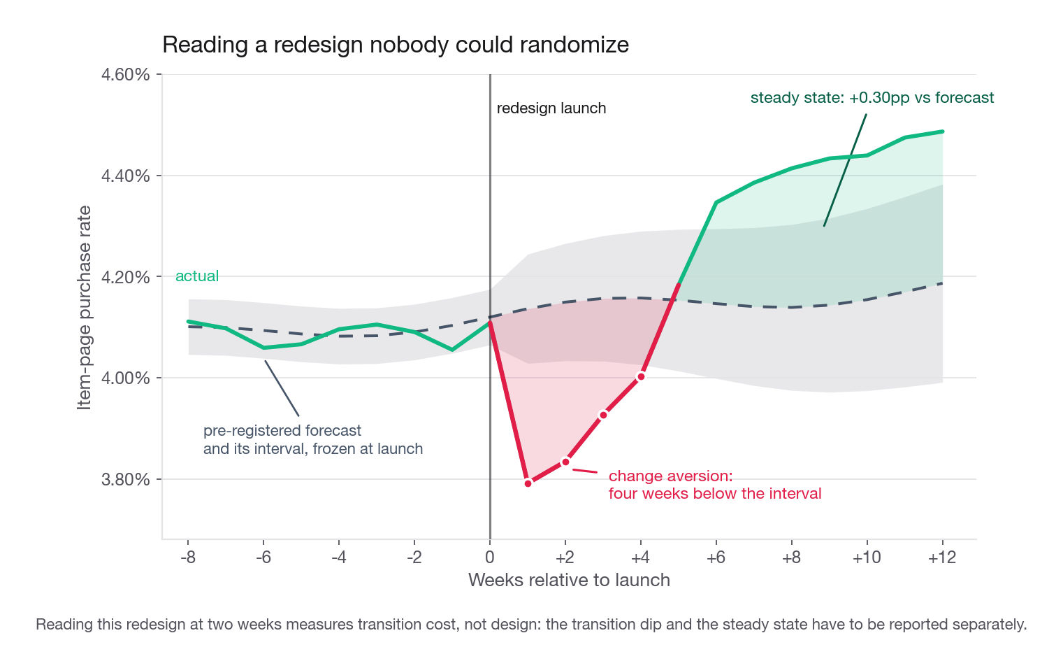
Pre-registration is what makes this respectable rather than a story. Anyone can fit a time-series model after a launch and produce a counterfactual that flatters it. Writing the forecast down first, with its interval, and showing the same model was right on three prior quiet windows, is the difference between an estimate and a narrative.
Two weaknesses to name first. One side of the comparison is a prediction, so it carries model error on top of sampling error and the interval is wide. That is tolerable because these changes are large: a rebrand that moves the north star by less than the forecast noise did not need measuring. And the estimate is fragile to anything else that week, so keep a log of concurrent launches, marketing spend, seasonality, and outages, and check it first when the number looks strange.
Change aversion
Small changes get flattered by novelty; large changes get punished by its mirror image. Users with muscle memory for the old item page will be slower and more frustrated on the new one for a while, regardless of quality. Read a redesign at two weeks and you are measuring transition cost, not design.
With three prior redesigns Halcyon has three decay curves and can estimate how deep the penalty goes and how long it lasts. Model it, subtract it, and report the transition number and the estimated steady state separately. With no prior data, wait six to ten weeks rather than two and weight tenured and brand-new cohorts separately, since a user who joined after the change has nothing to unlearn.
Further reading worth an evening
The most useful writing on this comes from teams publishing what they actually do. A short, opinionated list by purpose, with no links, because the useful ones are findable by name and the ephemeral ones are not worth chasing.
For how a platform is put together, Netflix has written repeatedly about assignment mechanics and platform internals, the part most write-ups skip in favour of statistics. Microsoft's experimentation group has published tutorials and a long rules-of-thumb paper built from thousands of real tests, including plenty of unflattering material about results that surprised them. That paper is the best available cure for over-confidence about effect sizes.
For the statistics of running many tests, Stitch Fix's engineering blog has an unusually clear practitioner treatment of multiple hypothesis testing, plus a companion piece on how the minimum detectable effect drives sample size. Google's data science blog makes the point that the effect size you care about is really a business parameter: a software company chases tiny gains because deployment is nearly free, while a company shipping physical goods or human services cannot.
For experiments where users are not independent, Instacart wrote the clearest thing available on why a marketplace breaks user-level randomization, including the options they rejected and why. Google covers geographic experiments and, separately, designing tests on a social graph where treatment leaks along connections. Read those alongside 5.1.
For things going wrong, Walmart's engineering team has written on monitoring and alerting to catch broken experiments early, unglamorous and probably the highest-value operational reading here. Google has a good piece on the mobile problem of users offered a new version who never install it. For the wider job, LinkedIn covers the full arc of a growth project including short-horizon proxies, which pairs with 5.2.
One caution. Engineering blogs are recruiting instruments as much as documentation, so expect a bias toward elaborate approaches and silence about the simple thing that actually shipped. When a post describes a complicated method, ask whether it ran longer than a quarter and whether it changed a decision.
Common traps
Treating Bonferroni as the answer rather than one answer. It controls the wrong error for a product program. On Halcyon's quarter it prevented four bad ships at the cost of fifteen good ones, and the nineteen-ship drop usually quoted instead double-counts those four fakes as part of the price. Fix: name the false discovery rate as the target, with Benjamini-Hochberg as the default and Bonferroni reserved for small pre-registered families and irreversible decisions.
Assuming concurrent tests contaminate each other. With independent assignment they do not bias anything, they add variance. Fix: explain why randomization balances the other tests across your arms, then note the exception is genuine interaction, handled by exclusivity layers rather than by testing.
Testing for interactions as a matter of routine. The interaction term carries twice the standard error of a main effect, so the check is badly underpowered and its null result means little. Fix: gate on product logic, force exclusivity where two changes touch the same element, and fund a factorial only when you genuinely expect an interaction.
Reading a marginal p-value as if it were the average winner. In Halcyon's program, results between 0.03 and 0.05 were real 54 percent of the time and results below 0.01 were real 93 percent. Fix: report effect size and interval, and note where in the winners distribution the result sits.
Chasing significance when the real problem is the prior. A team whose ideas work one time in ten cannot fix ship quality with a stricter alpha, it will just ship less of everything. Fix: quote the probability that a declared winner is real and point at idea quality and power as the two levers.
Two-arm testing a first-version machine-learned feature. The result mixes the model with the layout carrying it. Fix: three arms, with a third arm that is a weak model but a sane product.
Using random suggestions as the baseline arm. Statistically cleanest, and it poisons the users you want to measure, permanently. Fix: a non-learned rule that still looks reasonable, such as other titles by the same author.
Refitting the counterfactual model after an untestable launch. A model refit on post-launch data absorbs the effect and reports that roughly nothing happened. Fix: fit and freeze before launch, write down the predicted path and interval, and validate on prior quiet windows.
Reading a redesign at two weeks. You measure change aversion, not design quality, and you will roll back something that was working. Fix: estimate the transition penalty from past redesigns, report steady state separately, and cohort users who joined after the change.
Saying no to early stopping without offering an alternative. "The rules say three weeks" makes you an obstacle. Fix: explain the cost in plain terms, then propose a group sequential design with pre-specified looks so early stopping becomes legitimate rather than forbidden.
Quick self-check
Answer these out loud, in full sentences, as if the interviewer just asked them.
Thirty homepage variants, one wins at p equals 0.04. Give two independent reasons not to ship, one about multiplicity and one about what a marginal p-value is worth at modest power. Then say what you would do next.
Explain to a product manager with no statistics background why controlling the false discovery rate across a quarter beats controlling the chance of any single mistake. Use a concrete count of ships and errors.
Two experiments are live on the same item page, one changing sort order and one adding a price badge. Are the estimates biased? Say what randomization guarantees, what it does not, and how you decide whether to force exclusivity.
Your surface gets 9,000 eligible sessions a week and sizing says eleven weeks. Give four things you would try before calling the test impossible, and what each costs.
Design the test for a first-version recommendation shelf. Name the three arms, say exactly what populates the third, and state which two comparisons answer which two decisions.
Halcyon is replacing its wordmark and colour system next month. Describe how you would estimate the impact, name the one step that makes the estimate credible rather than a story, and say how you would separate transition cost from the steady-state effect.