4.2 Sample Size, Power, and How Long to Run
Find the core decision, design, or behavior signal.
Turn the lesson into a concise response blueprint.
Name the trap you would avoid in a real interview.
Use these checkpoints as your reading path before diving into the full lesson.
- 1Why this matters in interviews
- 2The four quantities, and the only one y...
- 3Significance level
- 4Power
- 5Baseline and its variance
The previous lesson got you to a hypothesis, a unit of randomization, a primary metric, and a written decision rule. This one answers the question the engineering manager asks thirty seconds later: how many users, and until when. The answer is not "two weeks" by reflex. By the end of this page you will be able to take a baseline rate, a business case, and a daily traffic number and say "we need 34,700 sessions per arm, which is thirteen days at a fifty-fifty split, so we run two full weeks and read it on a Monday", then defend every clause of that sentence.
Why this matters in interviews
Sizing is where interviewers find out whether you have shipped experiments or only read about them. The formula is a small part of it. What gets scored is the reasoning around the formula.
A weak answer: "I would use a power calculator with alpha of 0.05 and power of 0.8 and run it for two weeks." Every clause is defensible and none of it is an answer, because the candidate has not said what effect they are trying to detect, where that number came from, or what they would do if two weeks is not enough.
A strong answer runs the other direction. It starts from money: what improvement would make this worth building, given the build cost. Then it converts that improvement into a sample size, the sample size into days at real traffic, checks whether those days are a sane number of calendar weeks, and only then reports back. If the number is absurd, a senior candidate says so and proposes a different design rather than quietly running an underpowered test.
The second thing being scored is subtler. Sample size is a decision input, not a fact about the world. Every quantity in it is negotiable except one, and knowing which is fixed, which you own, and which the product manager owns is most of the job.
Interview tip: Open with "the sizing question is really a question about what lift is worth shipping, so let me start there" and you have already separated yourself from most of the pool.
The four quantities, and the only one you actually choose
Every power calculation, for any metric, is a relationship among four numbers. Fix any three and the fourth falls out. In practice you fix three by convention or measurement and solve for the fourth, which is why the exercise feels like a black box until you see which is which.
Significance level
The significance level, written alpha, is the rate at which you are willing to call a neutral change a winner. Set it to 0.05 and you accept that one in twenty tests of a change that does nothing will still cross the line and get shipped.
Lowering alpha to 0.01 makes you harder to fool and more expensive to satisfy. On the Larkspur numbers below it moves the requirement from 34,671 sessions per arm to 51,590, a 49 percent surcharge for one extra digit of caution. You almost never touch alpha in a single test. It moves when you are running many tests at once and want to control false launches across the whole program, which is the multiple-comparisons material later in this section.
Power
Power, written as one minus beta, is the probability that a real effect of the size you care about actually clears your bar. Power of 0.80 means that if the change truly delivers the improvement you specified, you will detect it four times out of five and miss it once out of five.
Candidates treat 0.80 as a law. It is a convention encoding "a missed winner is roughly four times cheaper than a false launch", and that trade is not always right for you. If the change is cheap and the downside of missing it is a competitor shipping first, 0.80 is too conservative. If it is a permanent architectural commitment, 0.90 is worth the extra data: on Larkspur that takes the requirement from 34,671 per arm to 46,414, a 34 percent surcharge.
Baseline and its variance
The third input is what the metric does today. For a proportion metric this is a single number, the current rate, and it pins the variance automatically: a rate of p has variance p times one minus p per observation. For a continuous metric like revenue per session you need the standard deviation separately, and this is where most sizing exercises fall apart.
The baseline is the one quantity you do not choose. Measure it from at least four full weeks of history, on exactly the population eligible for the test. Measuring it on all traffic and then running only on logged-in mobile users is a common and expensive mistake.
Minimum detectable effect
The minimum detectable effect, usually shortened to MDE, is the smallest improvement you insist on being able to see. This is the lever, and it is not a statistical question at all. It is a claim about what is worth your engineering time, your testing slot, and the risk of showing real users a worse experience, and that claim belongs to whoever owns the roadmap. Your job is to price it: hand back a table of what each candidate threshold costs in days.
| Input | Who owns it | Typical value | Effect of tightening it | Do you negotiate it |
|---|---|---|---|---|
| Significance level, alpha | Data science, as a program-wide default | 0.05 two-sided | 0.05 to 0.01 costs 49 percent more data | Rarely, and program-wide if so |
| Power, one minus beta | Data science, per test class | 0.80 | 0.80 to 0.90 costs 34 percent more data | Occasionally, for irreversible changes |
| Baseline rate and variance | Nobody, you measure it | 8.4 percent add-to-cart | Not adjustable | Never, but measure it on the right population |
| Minimum detectable effect | Product, informed by your cost table | 4 to 10 percent relative | Halving it costs four times the data | Always, and this is the whole conversation |
Interview tip: If you can only remember one line from this lesson, remember that alpha and power are conventions, the baseline is measured, and the MDE is a business decision that you price rather than pick.
The dataset behind every number on this page
The running example is Larkspur, an online outdoor-gear retailer. The metric is search-results-page to add-to-cart rate per session, and the block below builds twenty-eight days of pre-experiment session logs deterministically. One row is one session.
Say the assignment unit out loud first, because every number below depends on it. Larkspur randomizes at the session level, so the unit that gets assigned and the unit in the metric denominator are the same thing. That is deliberate and not the default. The previous lesson made the visitor the default for funnel changes and kept session assignment for surfaces with no memory across visits. The size-and-fit module does its whole job inside one visit, and the outcome is scored before the shopper leaves. The price is that a twice-visiting shopper can see both versions, tolerable here and not for pricing or onboarding. Every sample size on this page is therefore a session count.
import numpy as np
import pandas as pd

SEED = 71092026
rng = np.random.default_rng(SEED)

DAYS, BASE = 28, 5600
mult = np.array([1.06, 1.04, 1.02, 1.00, 1.09, 0.84, 0.79])[np.arange(DAYS) % 7]
counts = rng.poisson(BASE * mult)

day = np.repeat(np.arange(DAYS), counts)
n = day.size
weekend = np.isin(day % 7, [5, 6])

device = np.where(rng.random(n) < np.where(weekend, 0.71, 0.58), "mobile", "desktop")
country = rng.choice(["US", "CA", "UK", "AU"], n, p=[0.58, 0.14, 0.19, 0.09])
returning = rng.random(n) < np.where(weekend, 0.36, 0.47)

p = np.full(n, 0.0795)
p += np.where(device == "mobile", -0.021, 0.024)
p += np.where(returning, 0.033, -0.012)
p += np.where(country == "US", 0.004, -0.006)
added = rng.random(n) < p

order = added & (rng.random(n) < 0.42)
revenue = np.where(order, rng.gamma(2.0, 41.0, n), 0.0).round(2)

larkspur = pd.DataFrame({
    "session_id": np.arange(1, n + 1), "day": day, "device": device,
    "country": country, "is_returning": returning.astype(int),
    "added_to_cart": added.astype(int), "revenue": revenue,
})
print(larkspur.shape, round(larkspur["added_to_cart"].mean(), 5),
      int(round(len(larkspur) / DAYS)))
(153557, 7) 0.08413 5484Three numbers to hold onto: the baseline add-to-cart rate is 8.413 percent, average traffic is 5,484 sessions per day, and weekday and weekend behave differently, deliberately, because that difference drives the calendar section later.
Sizing a proportion metric by hand
You should be able to write the two-proportion sample size formula from memory, because interviewers ask you to explain it, not to run it.
The logic in words: you are comparing two rates, so your estimate of the difference carries a standard error built from both arms. The gap you care about has to sit far enough from zero that a null world rarely produces it, and far enough the other way that a true-effect world usually produces something past your threshold. The first requirement contributes a z value for alpha under the pooled rate, the second a z value for power under the two separate rates. Add those distances, divide by the effect you want to see, square it.
from scipy.stats import norm

def n_per_arm(p_base, lift_abs, alpha=0.05, power=0.80, sides=2):
    p_var = p_base + lift_abs
    p_pool = (p_base + p_var) / 2
    z_alpha = norm.ppf(1 - alpha / sides)
    z_beta = norm.ppf(power)
    spread = (z_alpha * np.sqrt(2 * p_pool * (1 - p_pool))
              + z_beta * np.sqrt(p_base * (1 - p_base) + p_var * (1 - p_var)))
    return int(np.ceil((spread / lift_abs) ** 2))

BASE_RATE = 0.0841
print("Larkspur, +0.60pp:", n_per_arm(BASE_RATE, 0.0060))
print("textbook check   :", n_per_arm(0.10, 0.01))
Larkspur, +0.60pp: 34671
textbook check : 14751The second line is a habit worth keeping: verify against a case with a known answer. A 10 percent baseline with a one-point absolute lift is the canonical example, and the accepted answer sits just under 14,800 per arm. Matching it proves your code is not silently off by a factor of two, the most common bug in hand-rolled sizing.
The whiteboard version drops the two-variance refinement: n per arm equals two times the squared sum of the two z values, times the pooled rate times one minus the pooled rate, over the squared absolute lift. On Larkspur that gives 34,672 instead of 34,671. Use the simple form by hand, the exact form in code. Libraries exist too, and the common Python one parameterizes the effect through an arcsine transform, so it lands a percent or so away. Either is fine. What is not fine is quoting a web calculator and being unable to say what it did.
The formula counts independent units
One assumption is buried in that derivation and it is the one that bites in review. The formula treats every row as an independent draw, so it holds only when the thing you randomized and the thing you count are the same thing. At Larkspur they are, sessions assigned and sessions counted, so 34,671 stands.
Change the assignment unit and the arithmetic moves underneath you. Randomize by visitor while still measuring add-to-cart per session, and two sessions from one shopper are not two independent observations, because a shopper who adds to cart once tends to do it again. Inflate the requirement by the design effect: DEFF equals one plus average sessions per visitor minus one, times the within-visitor intraclass correlation of the outcome.
iid_per_arm = n_per_arm(BASE_RATE, 0.0060)
for m_bar, rho in ((3, 0.15), (3, 0.30), (3, 0.60)):
    deff = 1 + (m_bar - 1) * rho
    per_arm = int(np.ceil(iid_per_arm * deff))
    days = 2 * per_arm / 5484
    print(f"m={m_bar} rho={rho:.2f}  DEFF {deff:.2f}  {per_arm:>7,}/arm  "
          f"{days:5.1f} days  ->  {int(np.ceil(days / 7)) * 7} run days")
m=3 rho=0.15 DEFF 1.30 45,073/arm 16.4 days -> 21 run days
m=3 rho=0.30 DEFF 1.60 55,474/arm 20.2 days -> 21 run days
m=3 rho=0.60 DEFF 2.20 76,277/arm 27.8 days -> 28 run daysThe previous lesson measured this and got a standard error 1.49 times wider once it clustered on the visitor, a variance ratio of 2.2. Treat that as one measurement, not a constant: the bottom row above reproduces 2.2 at three sessions per visitor with a correlation of 0.60, and halving that correlation drops the surcharge to 1.60.
Read the run-days column. At a design effect of 2.2 the Larkspur plan is not thirteen days, it is 27.8, which rounds to four full weeks. That beats the alpha surcharge of 1.49 times and the power surcharge of 1.34 times, both of which this page prices out loud, and it is the one that routinely goes unpriced.
Two refinements. Kish assumes every visitor contributes the same number of sessions, and real counts are skewed, so it understates: replace the average with the average times one plus the squared coefficient of variation of per-visitor session counts, or read the empirical variance ratio straight off an A/A test instead. The cleaner move is to size on the assignment unit from the start, making the metric the share of visitors who added to cart, at which point the design effect disappears.
Absolute versus relative, and why calculators disagree
This is where real sizing errors come from. An absolute lift is measured in percentage points, a relative lift as a fraction of the baseline. On an 8.41 percent baseline a 0.60 point absolute gain is a 7.1 percent relative gain. Same event, two descriptions, and feeding one into a calculator that expects the other puts you off by more than an order of magnitude. Product managers speak in relative terms almost always: "lift conversion 5 percent" means multiply the rate by 1.05. The formula wants absolute. Convert explicitly, out loud, every time.
| Baseline rate | A 5 percent relative lift equals | A 0.5 point absolute lift equals | Sessions per arm for the relative version |
|---|---|---|---|
| 2.0 percent | 0.10 points | 25 percent relative | 306,000 |
| 8.4 percent | 0.42 points | 5.9 percent relative | 69,900 |
| 25.0 percent | 1.25 points | 2.0 percent relative | 19,300 |
| 60.0 percent | 3.00 points | 0.8 percent relative | 4,500 |
Read the last column. The same relative ambition costs sixty-eight times more traffic on a 2 percent baseline than on a 60 percent one. That is why testing something rare, a purchase or a subscription upgrade, is so much harder than testing a click, and why teams that only ever test deep-funnel metrics are chronically underpowered.
Interview tip: When an interviewer says "detect a 5 percent improvement", ask "5 percent relative or half a point absolute" before you compute anything. It takes four seconds and it is a senior signal.
The inverse square law
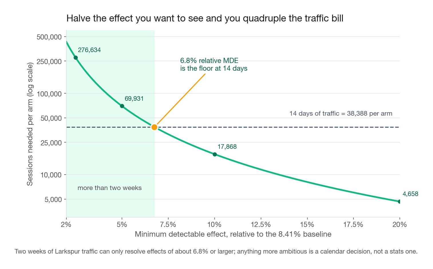
Look at the denominator. The effect size is squared, and every fact about experiment economics follows from that exponent. Halve the effect you want to detect and you quadruple the sample. Cut it to a third and you need nine times the data. That is why a 5 percent MDE means a month-long test and a 10 percent MDE means a week-long one.
DAILY = 5484
for rel in (0.025, 0.05, 0.075, 0.10, 0.15, 0.20):
    lift = BASE_RATE * rel
    per_arm = n_per_arm(BASE_RATE, lift)
    days = 2 * per_arm / DAILY
    print(f"{rel:6.1%} {lift * 100:7.3f}pp {per_arm:10,} {2 * per_arm:11,} {days:8.1f}")
2.5% 0.210pp 276,634 553,268 100.9
5.0% 0.420pp 69,931 139,862 25.5
7.5% 0.631pp 31,423 62,846 11.5
10.0% 0.841pp 17,868 35,736 6.5
15.0% 1.261pp 8,111 16,222 3.0
20.0% 1.682pp 4,658 9,316 1.7That table is the most useful artifact you can hand a product manager, and producing it unprompted is worth more in an interview than deriving the formula, because it converts an argument about ambition into a schedule. A PM who wants to detect a 2.5 percent relative gain is asking for a fourteen-week test on this traffic. Once "fourteen weeks" is sitting next to the number, the conversation about whether 7.5 percent is the more honest threshold happens by itself.
Halving a confidence interval costs four times the data
The same exponent runs the other direction, and this version is a stock rapid-fire question: someone shows you an interval too wide to act on and asks what it takes to tighten it. The half-width on a difference in proportions is a z value times the standard error, and the standard error carries a square root of n in the denominator, so the interval shrinks with the square root of the sample. Half as wide costs four times the data. A third as wide costs nine times.
z_crit = norm.ppf(0.975)
for per_arm in (8_668, 17_336, 34_671, 69_342, 138_684):
    half = z_crit * np.sqrt(2 * BASE_RATE * (1 - BASE_RATE) / per_arm)
    print(f"{per_arm:>9,}  +/- {half * 100:.4f} pp  ({half / BASE_RATE:.2%} relative)")
8,668 +/- 0.8263 pp (9.82% relative)
17,336 +/- 0.5843 pp (6.95% relative)
34,671 +/- 0.4131 pp (4.91% relative)
69,342 +/- 0.2921 pp (3.47% relative)
138,684 +/- 0.2066 pp (2.46% relative)Each row quadruples the sample of the row two above it and exactly halves the interval. Say it as "precision scales with the square root of sample size, so halving the interval is a four-fold cost", then give the numbers.
The corollary is the part juniors miss. Because precision gets expensive so fast, the cheapest way to tighten an interval is rarely more traffic, it is less noise. A metric with more events per user, capped outliers, or pre-experiment behavior regressed out can each halve the variance, worth as much as doubling the run length at no calendar cost.
Choosing the minimum detectable effect from business value
Here is the part that separates candidates. Almost everyone can run the calculator. Very few can say where the MDE came from without using the word "reasonable".
The MDE has a floor and a ceiling, and both are computable.
The floor: what lift pays for the build
The floor is the smallest improvement worth having. Below it, even a real and statistically clean win loses money once you count the build and maintenance cost.
Work it out for Larkspur. The change under test is a redesigned size-and-fit module on the search results page: six weeks across three engineers plus maintenance, booked at roughly 48,000 dollars in year one. Each extra add-to-cart is worth average order value times contribution margin times the probability that a cart becomes an order.
AOV = 74.0
MARGIN = 0.22
CART_TO_ORDER = 0.42
value_per_add = AOV * MARGIN * CART_TO_ORDER
annual_sessions = DAILY * 365
build_cost = 48_000.0

mde_floor = build_cost / (annual_sessions * value_per_add)
print("value of one added cart :", round(value_per_add, 2))
print("annual sessions         :", annual_sessions)
print("value of +1.00pp per yr :", round(annual_sessions * 0.01 * value_per_add))
print("MDE floor               :", round(mde_floor * 100, 3), "pp =",
      round(mde_floor / BASE_RATE * 100, 2), "% relative")
print("sample per arm at floor :", f"{n_per_arm(BASE_RATE, mde_floor):,}")
value of one added cart : 6.84
annual sessions : 2001660
value of +1.00pp per yr : 136866
MDE floor : 0.351 pp = 4.17 % relative
sample per arm at floor : 100,165Now you have a sentence worth saying. One percentage point of add-to-cart rate is worth about 137,000 dollars a year at Larkspur, so a 48,000 dollar build breaks even at 0.35 points, a 4.2 percent relative lift. Detecting anything smaller is pointless, because you would not ship it anyway.
Detecting exactly 4.2 percent takes 100,165 sessions per arm, 200,330 total, which at 5,484 per day is thirty-seven days. That is uncomfortable, which is why it is worth saying. Five and a half weeks of a slot to detect the break-even effect is a bad trade, because the slot has an opportunity cost: the next three experiments you did not run.
So the floor is where you start, not where you land. Set the MDE above break-even, often at one and a half to two times it, and name the consequence rather than hiding it: you are choosing not to detect wins in the 4 to 7 percent band.
The ceiling: what lift is even plausible
The ceiling comes from history. Pull the last twenty or thirty shipped experiments on this surface and look at the measured effects. On a mature checkout funnel the median shipped win is usually 1 to 3 percent relative, and a 15 percent win happens once every couple of years.
If your MDE is 15 percent because that is what fits in two weeks, you have designed a formality that will come back neutral and teach you nothing, because the smallest effect you can see is larger than any effect this product has produced. That is worse than not testing: it consumes the slot and manufactures a false sense of rigor. If the floor sits above the ceiling, the correct recommendation is to not run the test, and to say why.
Traffic allocation: splits, ramps, and the harmonic mean penalty
Sample size tells you how many sessions each arm needs, allocation tells you how fast you accumulate them. Three regimes cover almost every real case, and interviewers like to move you between them mid-question.
| Situation | Daily eligible traffic | Total needed at 7.1 percent MDE | What you do |
|---|---|---|---|
| Tandem, a B2B invoicing tool | 1,900 sessions | 70,000 | 37 days at fifty-fifty, so either raise the MDE, pick a higher-frequency metric, or accept a six-week test |
| Larkspur, mid-size retail | 5,484 sessions | 70,000 | 13 days at fifty-fifty, so run fifty-fifty and read at two full weeks |
| Northgate, a large marketplace | 480,000 sessions | 70,000 | 4 hours at fifty-fifty, so hold it to about 1 percent of traffic and still run two full weeks |
The Northgate row is the counterintuitive one. When traffic is abundant the binding constraint stops being sample and becomes calendar and risk. You still want two weeks of clock time for the weekly cycle, but not half a million users a day on an untested experience when 1 percent answers the question. This is why large platforms run most experiments on single-digit percentages, and why "what share of traffic" and "for how long" are two decisions, not one.
Ramping is the standard resolution: 1 percent for a day to catch crashes, then 5 percent, then your target allocation. Count only sessions collected at stable allocation.
Why unequal splits cost more than they look
A common request is 90 percent control and 10 percent treatment because the treatment is risky. That is a legitimate risk decision with a steep price, and you should quote the price. Effective sample size for a two-arm comparison is the harmonic mean of the arm sizes, not the total, and the penalty relative to an even split is one quarter divided by the product of the two shares.
for share in (0.50, 0.40, 0.30, 0.20, 0.10, 0.05):
    print(f"{share:.0%}/{1 - share:.0%}   x{0.25 / (share * (1 - share)):.2f}")
50%/50% x1.00
40%/60% x1.04
30%/70% x1.19
20%/80% x1.56
10%/90% x2.78
5%/95% x5.26Sixty-forty is nearly free at 4 percent extra. Ninety-ten costs 2.78 times the traffic for the same power, turning a thirteen-day test into a thirty-six-day one. The right way to hold that conversation: "a 10 percent treatment arm is fine for the first two days as a safety ramp, and if we keep it there for the whole test we need thirty-six days instead of thirteen. Which do you want."
Interview tip: Quoting the harmonic-mean penalty for a 90/10 split from memory, 2.78 times, is one of the highest-signal small facts in experimentation interviews.
Why the calendar matters as much as the count
Sample size is necessary and not sufficient. A test that collects the right number of sessions over the wrong span of days answers a question nobody asked.
Whole weeks, always
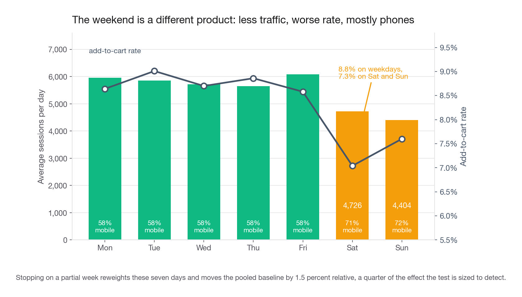
Larkspur's Tuesday and its Saturday are different products with different users.
by_dow = larkspur.groupby(larkspur["day"] % 7).agg(
    sessions=("session_id", "size"),
    add_rate=("added_to_cart", "mean"),
    mobile_share=("device", lambda s: (s == "mobile").mean()),
)
print(by_dow.round(4))
sessions add_rate mobile_share
day
0 23829 0.0864 0.5795
1 23421 0.0901 0.5784
2 22861 0.0870 0.5778
3 22613 0.0886 0.5766
4 24314 0.0858 0.5794
5 18904 0.0704 0.7132
6 17615 0.0760 0.7156Weekday add-to-cart sits near 8.8 percent, weekend near 7.3 percent, and mobile share jumps from 58 to 71 percent on the weekend. The two facts are connected: weekend traffic is more mobile, and mobile converts worse here. Now watch what happens if you stop on a convenient-looking day rather than a week boundary.
for cut in (12, 13, 14, 15, 16):
    part = larkspur[larkspur["day"] < cut]
    print(cut, f"{len(part):,}", round(part["added_to_cart"].mean(), 5))
12 68,021 0.08609
13 72,662 0.08512
14 77,142 0.08479
15 82,966 0.08505
16 88,787 0.08528Day twelve gives 8.609 percent, day fourteen gives 8.479 percent. That 0.13 point gap is 1.5 percent relative and it is pure calendar composition: twelve days from a Monday hold ten weekdays and two weekend days instead of the natural five-to-two ratio.
Now put it next to the MDE. You are trying to detect 0.60 points, and a stopping-day artifact worth 0.13 points is over a fifth of the signal, injected by nothing but arithmetic. In a randomized test both arms absorb the same shift so it mostly cancels, and "mostly" is doing real work there: it stops cancelling the moment allocation is uneven across days, a ramp finishes mid-week, or one arm's caching interacts with weekday traffic. The rule is multiples of seven. If sizing says 13 days, run 14. If it says 16, run 21. The extra days are cheap and the alternative is an argument you cannot win.
The population changes while the test runs
There is a second calendar effect with nothing to do with weekdays, and it does not care what you randomized. Whatever the assignment unit, the pool on day one is dominated by your most frequent users, because frequent users show up first. Larkspur's session-level test is no exception: day-one sessions are disproportionately produced by heavy shoppers. By day fourteen the pool includes occasional visitors. Those groups convert differently, so the effect measured on day three sits on a different population than the effect measured on day fourteen, even with perfect randomization and no novelty effect at all.
So early readings are not merely noisy, they are biased toward whatever your heaviest users do. If the treatment helps power users and hurts casual ones, a three-day read looks great and a three-week read looks neutral. This is distinct from novelty and primacy effects, which concern behavior changing rather than who is in the sample, and which get their own lesson shortly. The defense is the same as for weekly cycles: fix the run length before launch, and until you reach it monitor guardrails and instrumentation health, not the primary metric.
Interview tip: Say "a fourteen-day test is not a seven-day test run twice, because the population composition differs" and you will get a follow-up question you are prepared for.
Continuous metrics: variance is the whole problem
Everything so far assumed a proportion, where the baseline pins the variance. Revenue per session does not, and interviewers use it to see whether you understood the formula or memorized it. The structure is identical: two z values, squared, times variance, divided by the squared effect. The difference is that variance is now an independent input you must measure, and for revenue it is enormous.
mu = larkspur["revenue"].mean()
sd = larkspur["revenue"].std()
cap = larkspur["revenue"].quantile(0.99)
wins = larkspur["revenue"].clip(upper=cap)

def n_continuous(mean, stdev, rel_lift, alpha=0.05, power=0.80):
    z_a = norm.ppf(1 - alpha / 2)
    z_b = norm.ppf(power)
    return int(np.ceil(2 * (z_a + z_b) ** 2 * stdev ** 2 / (rel_lift * mean) ** 2))

print("raw    mean", round(mu, 3), "sd", round(sd, 2), "CV", round(sd / mu, 2))
print("capped mean", round(wins.mean(), 3), "sd", round(wins.std(), 2),
      "CV", round(wins.std() / wins.mean(), 2), "cap at", round(cap, 2))
for rel in (0.02, 0.03, 0.05):
    print(f"{rel:.0%} lift -> raw {n_continuous(mu, sd, rel):,} vs capped "
          f"{n_continuous(wins.mean(), wins.std(), rel):,} per arm")
raw mean 2.877 sd 18.44 CV 6.41
capped mean 2.358 sd 13.64 CV 5.78 cap at 101.93
2% lift -> raw 1,612,538 vs capped 1,312,499 per arm
3% lift -> raw 716,684 vs capped 583,333 per arm
5% lift -> raw 258,006 vs capped 210,000 per armThe coefficient of variation, standard deviation over mean, is 6.41, and that one number explains why revenue tests are so hard: most sessions produce zero and a handful produce hundreds of dollars, so the metric is almost all noise. Detecting a 2 percent lift in revenue per session needs 1.6 million sessions per arm, or 588 days. The same 2 percent on add-to-cart rate, coefficient of variation near 3.3, needs 434,000.
Capping at the 99th percentile cuts the requirement about 19 percent. Real, but not a rescue, and it introduces bias: you are now measuring censored revenue, so a treatment that works by producing more very large orders reads as neutral. Say that trade out loud rather than presenting capping as free.
| Metric on the same sessions | Coefficient of variation | Sessions per arm for a 2 percent relative lift | Days at 5,484 per day, fifty-fifty |
|---|---|---|---|
| Add-to-cart rate | 3.3 | 434,000 | 158 |
| Revenue per session, capped at p99 | 5.8 | 1,312,000 | 479 |
| Revenue per session, raw | 6.4 | 1,613,000 | 588 |
The honest read is that Larkspur cannot run a revenue-per-session test at all. Make revenue a guardrail with a wide non-inferiority band, power the test on add-to-cart, and argue the revenue case from the funnel rather than from the experiment. That is not a dodge, it is the answer.
Variance reduction is the other lever and is worth one sentence because it shows range. Regressing out pre-experiment revenue for the same users, the technique commonly called CUPED, typically removes 30 to 50 percent of variance on metrics with strong week-to-week autocorrelation, equivalent to 40 to 100 percent more sample for free. It does nothing for brand-new users, who have no history, so its value tracks how much of your traffic is returning.
When the right answer is "do not run this test"
An underpowered test is not a weak test, it is an actively misleading one, and this is the part of sizing candidates almost never mention.
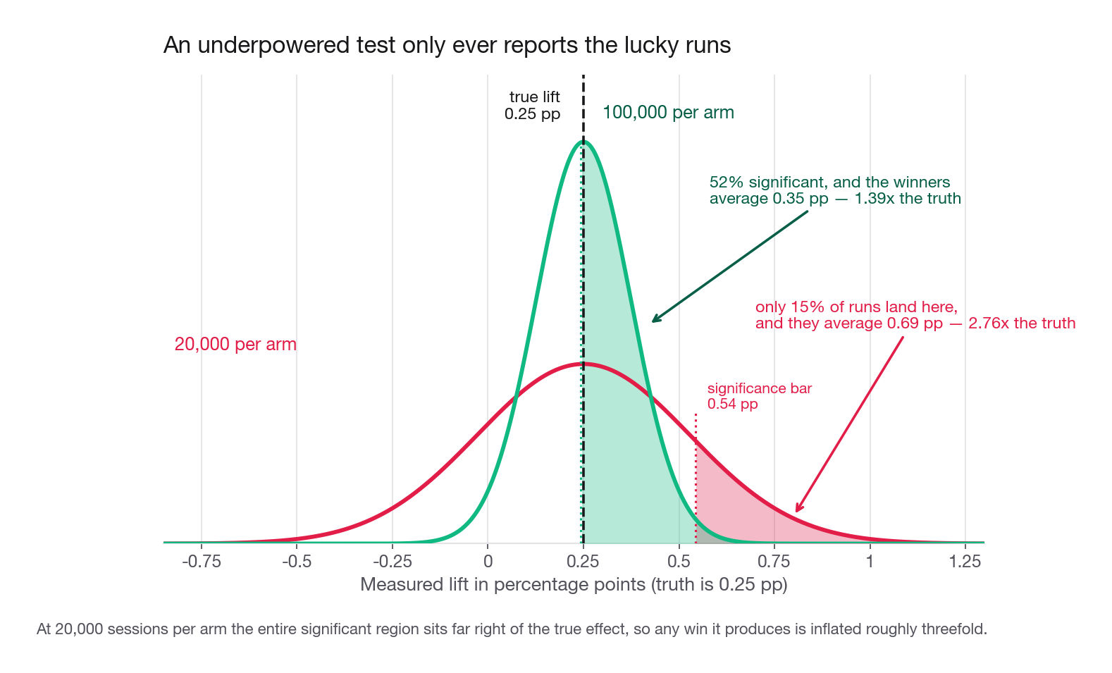
Suppose the true effect at Larkspur is a 3 percent relative lift, 0.25 points, and you run 20,000 sessions per arm because that is what a week gives you. Power is 15 percent, so most of the time you get nothing. The interesting question is what happens the one time in seven that you cross the threshold.
sim = np.random.default_rng(4409)
TRUE_LIFT = 0.0025

def replicate(per_arm, reps=200_000):
    a = sim.binomial(per_arm, BASE_RATE, reps) / per_arm
    b = sim.binomial(per_arm, BASE_RATE + TRUE_LIFT, reps) / per_arm
    diff = b - a
    pooled = (a + b) / 2
    se = np.sqrt(2 * pooled * (1 - pooled) / per_arm)
    hit = np.abs(diff) > z_crit * se
    won = hit & (diff > 0)
    return hit.mean(), diff[won].mean() / TRUE_LIFT

for per_arm in (20_000, 34_671, 100_000):
    rate, exagg = replicate(per_arm)
    print(f"{per_arm:>8,}  significant {rate:5.1%}  average winner overstates by {exagg:.2f}x")
20,000 significant 14.7% average winner overstates by 2.76x
34,671 significant 21.8% average winner overstates by 2.15x
100,000 significant 51.6% average winner overstates by 1.39xRead the last column. At 20,000 per arm, when the test does declare a winner, the measured lift averages 2.76 times the truth. You report an 8 percent gain on a change that delivers 3 percent, the finance model gets built on 8 percent, and next quarter someone asks why the revenue never showed up.
This is the winner's curse, and it is mechanical, not a sign of anything malfunctioning. To clear a significance bar with a small sample the estimate has to be large, so the only estimates that survive are the lucky ones. The lower the power, the more extreme the survivors.
When sizing says a test is not viable, the options in rough order of preference are: raise the MDE by targeting a bigger change; move to a higher-frequency proxy metric earlier in the funnel and validate its link to the downstream metric separately; pool traffic across surfaces or geographies if the change is uniform; extend into a multi-week window if the slot is genuinely free; or ship on judgment with a monitoring plan and an explicit rollback trigger, saying plainly that this decision was made without experimental evidence.
That last one is a legitimate senior answer. Not everything can be tested, and pretending an underpowered test is evidence is worse than admitting you shipped on judgment.
Interview tip: Add "and if power comes out under 50 percent I would not run it, because a significant result would overstate the effect by two to three times" to any sizing answer. Almost nobody says it.
Common traps
Feeding a relative lift into a formula that wants an absolute one. A "5 percent lift" on an 8.4 percent baseline is 0.42 points, not 5 points, and getting it backwards changes the answer by roughly a factor of 140. Fix: write the absolute number down before touching a calculator, and state both when you report.
Measuring the baseline on the wrong population. Sizing on site-wide conversion and then testing only logged-in mobile users gives you a baseline, a variance, and a traffic number that are all wrong. Fix: compute the baseline with the exact eligibility filter the assignment code uses.
Sizing with the total sample instead of the per-arm sample. Every formula here returns sessions per arm, and halving your requirement by accident is the classic bug. Fix: sanity-check against a known case, such as a 10 percent baseline with a one-point lift needing about 14,750 per arm.
Stopping on a partial week. Composition alone moves the Larkspur baseline 1.5 percent relative between a twelve-day and a fourteen-day window. Fix: run multiples of seven days, rounding up.
Sizing on a metric whose variance you never measured. Proportions give variance for free, and people carry that habit into revenue, session length, and counts, where it is badly wrong. Fix: compute the standard deviation on real data and look at the coefficient of variation first.
Choosing the MDE so the test fits the calendar. The most common self-deception in experimentation. If the only detectable effect is larger than anything the product has produced, the test cannot succeed. Fix: derive the MDE from cost and history, then let the calendar be the output.
Reporting an underpowered win at face value. At 15 percent power the average significant result is nearly three times the truth. Fix: report power alongside the result, and shrink the forecast toward the prior when power was low.
Quoting a sample size without a date. "We need 70,000 sessions" does not answer "when can we decide". Fix: convert to days at the actual allocated traffic, round to weeks, name the read date.
Quick self-check
Answer these out loud, in full sentences, the way you would on a loop.
Your baseline conversion rate is 4 percent and the PM asks for the sample size to detect a 10 percent improvement. What do you ask before computing, what absolute lift do you use, and roughly how does the requirement compare to the same request on a 20 percent baseline?
A stakeholder shows you a result whose 95 percent interval runs from minus 1.1 points to plus 2.3 points and asks what it would take to cut that width in half. Give the factor, the reason, and one way to get there without more traffic.
Engineering will spend 48,000 dollars building a feature, and one point of conversion is worth 137,000 dollars a year. Walk through the break-even lift, then explain why you would set the MDE above it rather than at it.
The only test that fits your traffic has 20 percent power. The PM says "let us run it anyway, worst case we learn nothing". What is wrong with that reasoning, and what three alternatives do you propose?
Your primary metric is revenue per session with a coefficient of variation of 6.4. Explain in two sentences why that is harder to test than a conversion rate, and describe the design you would propose instead.