5.2 Long-Term Metrics, Opportunity Cost, and Reruns
Find the core decision, design, or behavior signal.
Turn the lesson into a concise response blueprint.
Name the trap you would avoid in a real interview.
Use these checkpoints as your reading path before diving into the full lesson.
- 1Why this matters in interviews
- 2Three different problems that sound ide...
- 3The running example
- 4Surrogate metrics: what actually makes...
- 5The two conditions
Some of the changes you most want to evaluate pay off on a horizon nobody will let you wait for. A subscription bundle is supposed to lift retention a year out. Meanwhile the experiment burns money every day it runs, and half the results you get back are statistically significant and commercially worthless. This lesson covers the three decisions in that gap: what you measure when the real outcome arrives too late, how long you leave people in an arm you already suspect is losing, and when it is honest to run the same test a second time.
Why this matters in interviews
The previous lesson covered the case where you cannot randomize at all. This one covers the case where randomization is fine and time is the enemy, and it separates two kinds of candidate cleanly.
The weaker candidate treats it as a power calculation, notices the run needs twelve months of exposure, and either proposes running it for twelve months or waves at "a proxy" without saying what makes a proxy trustworthy.
The stronger candidate treats time as a resource with a price. Every week the test runs, some population sits in the worse arm, and you can put a number on that. Every week you delay a winner you forgo its value, and you can price that too. A short-window metric is not a compromise, it is a modeling problem with a validation procedure attached, and if you cannot describe the validation you have not solved anything.
Three prompts collapse into this one skill:
We changed something whose payoff arrives in a year. How would you test it.
The test won with a good p-value. Why might you still not ship it.
We ran this test two years ago and it lost. Should we run it again.
Interview tip: Open any long-horizon question by naming the two costs explicitly, the cost of running and the cost of waiting, then say you will pick a horizon that minimizes their sum. That framing alone moves you a level.
Three different problems that sound identical
Candidates blur these together and then apply the wrong fix. Separate them out loud in the first minute.
| The problem | What it sounds like | Why the textbook test fails | First move |
|---|---|---|---|
| The metric matures slowly | "Does this lift twelve-month retention" | The label does not exist for a year, so no run length helps | Build and validate a short-window surrogate |
| The effect matures slowly | "Does this build a habit" | The label exists weekly, but the treatment effect has not converged in two weeks | Extend the run, cohort by exposure date, watch the effect curve flatten |
| The verdict is cheap but the change is expensive | "It won by 0.3 percent, do we build it" | Nothing is wrong with the test, the answer is an economics question | Compare annualized value against build and carry cost |
The middle row is the one people misdiagnose. If your metric is weekly workouts you can read it on day seven, but the day-seven effect is not the one you will live with, because novelty and primacy bend the early curve. The fix is cohorting on first exposure, not surrogacy. Do not reach for a predictive model when the honest answer is "run it four more weeks and read the cohort curves". The first row is the genuine surrogate problem, and it is where most of this lesson lives.
The running example
Ridgeline is a fictional subscription fitness app with about 2.1 million active members, paying 14 per month or 119 a year. The executive metric is twelve-month retention, the share of members still paying on the anniversary of their first charge, currently near 37 percent. The team wants to test a redesigned first-week onboarding: a guided plan builder, a coach introduction, a nudge to add one friend. Nobody will fund a fourteen-month experiment to find out whether it works.
Everything below runs on a synthetic table of a historical cohort, members who joined more than thirteen months ago so their outcome is known, with first-week behavior recorded alongside. This block builds it deterministically.
import numpy as np
import pandas as pd

SEED = 20260113
rng = np.random.default_rng(SEED)
sig = lambda z: 1 / (1 + np.exp(-z))

N = 40_000
plan = rng.choice(["monthly", "annual"], N, p=[0.72, 0.28])
channel = rng.choice(["organic", "paid_search", "paid_social", "referral"], N,
                     p=[0.31, 0.27, 0.28, 0.14])
market = rng.choice(["US", "CA", "GB", "AU"], N, p=[0.55, 0.14, 0.20, 0.11])

pull = {"organic": 0.35, "paid_search": 0.0, "paid_social": -0.45, "referral": 0.55}
fit = (rng.normal(0, 1, N) + np.array([pull[c] for c in channel])
       + 0.40 * (plan == "annual"))

w1_days = rng.binomial(7, sig(0.85 * fit - 0.55))
w1_workouts = rng.poisson(np.exp(0.15 + 0.55 * fit)) * (w1_days > 0)
w1_custom = (rng.random(N) < sig(0.9 * fit - 0.30)).astype(int)
w1_friend = (rng.random(N) < sig(0.7 * fit - 1.60)).astype(int)
w1_cancel = (rng.random(N) < sig(-1.2 * fit - 2.85)).astype(int)

logit12 = (-1.55 + 0.62 * fit + 0.11 * w1_days + 0.045 * w1_workouts
           + 0.30 * w1_custom + 0.42 * w1_friend - 2.1 * w1_cancel
           + 0.55 * (plan == "annual") + rng.normal(0, 0.9, N))
m12_retained = (rng.random(N) < sig(logit12)).astype(int)

ridgeline = pd.DataFrame({
    "member_id": np.arange(1, N + 1), "plan": plan, "channel": channel, "market": market,
    "w1_days_active": w1_days, "w1_workouts": w1_workouts,
    "w1_customized_plan": w1_custom, "w1_added_friend": w1_friend,
    "w1_cancelled": w1_cancel, "m12_retained": m12_retained,
})
print(ridgeline.shape, round(ridgeline["m12_retained"].mean(), 4))
(40000, 10) 0.3669One row is one member. Six columns describe the first seven days after signup. One column, m12_retained, is the thing you care about and cannot observe for a year.
Surrogate metrics: what actually makes one valid
A surrogate is a quantity you can read in days that you are willing to treat as a stand-in for the outcome you can read in months. Most candidates get half of the definition and it is the wrong half.
The two conditions
Condition one: the surrogate predicts the outcome. Members with a high surrogate value retain better than members with a low one. Everyone states this one and it is easy to check.
Condition two: the treatment's effect on the outcome runs entirely through the surrogate. If your change can reach twelve-month retention by any path that does not pass through the short-window behavior you measure, the surrogate will lie to you about that change specifically. Nobody mentions this one unprompted, and it is the condition that decides whether your test is trustworthy.
In interview language: a good surrogate is not merely correlated with the outcome, it has to carry the treatment effect. Correlation makes it a scoring tool. Mediation makes it a measuring instrument. Different jobs, and one does not imply the other.
Condition one is the easy half
Fit a model on the historical cohort predicting the known twelve-month label from first-week behavior only.
from sklearn.linear_model import LogisticRegression
from sklearn.model_selection import train_test_split
from sklearn.metrics import roc_auc_score, brier_score_loss

feat = ["w1_days_active", "w1_workouts", "w1_customized_plan",
        "w1_added_friend", "w1_cancelled"]
X = pd.get_dummies(ridgeline[feat + ["plan"]], columns=["plan"],
                   drop_first=True).astype(float)
y = ridgeline["m12_retained"]

Xtr, Xte, ytr, yte = train_test_split(X, y, test_size=0.30,
                                      random_state=7, stratify=y)
model = LogisticRegression(max_iter=1000).fit(Xtr, ytr)
p = model.predict_proba(Xte)[:, 1]
print("AUC", round(roc_auc_score(yte, p), 4),
      "Brier", round(brier_score_loss(yte, p), 4))
AUC 0.7352 Brier 0.1956An AUC of 0.735 from seven days against a twelve-month label is real signal and roughly what a subscription product should expect. Above 0.80 from a one-week window, check for leakage.
Ranking is not enough, because you will compare average predicted probability between arms, so the model has to be calibrated too. Bin the held-out scores into deciles and the predicted and actual rates track within about two points in every bin, with the top decile retaining at 71.6 percent against a 36.7 percent base and the bottom at 7.8 percent. That 9x spread is calibrated enough for the arm-level average to mean something.
Now look at what happens if you skip the model and use the obvious single-variable proxy instead.
| Candidate short-window proxy | Population share | Retention if true | Retention if false | AUC |
|---|---|---|---|---|
| Did not cancel in week 1 | 91.8 percent | 39.5 percent | 4.8 percent | 0.556 |
| Active on 3 or more days | 55.8 percent | 47.9 percent | 22.5 percent | 0.635 |
| Completed 2 or more workouts | 39.2 percent | 49.4 percent | 28.5 percent | 0.607 |
| Model score on all six columns | continuous | top decile 71.6 percent | bottom decile 7.8 percent | 0.735 |
The first row is the trap. Week-one cancellation looks devastating, 4.8 percent against 39.5 percent, and a candidate who sees that contrast declares victory. But it touches only 8.2 percent of members, so as a population-level instrument its AUC is 0.556, barely better than a coin. A surrogate that separates a tiny group spectacularly is a fine targeting rule and a poor measuring stick, because most of the effect you want to detect happens among the 92 percent it cannot distinguish.
Interview tip: When you propose a proxy, quote the conditional contrast and the share of the population it applies to together, because a candidate who quotes only the contrast has nothing to say about the other ninety percent.
Condition two is where surrogates die
Take the fitted Ridgeline surrogate, simulate five treatments against the same generative process, and compare what the surrogate says happened against what actually happened to twelve-month retention. Each arm reuses one random stream so arms differ only by the treatment, and the truth column is expected retention rather than a redrawn coin flip, which at 40,000 per arm would add about 0.7 points of noise and swamp the smallest effect on the board.
# Each arm rebuilds week one from the same generative equations, scores it with
# the frozen surrogate, and reads true retention as sig(logit12).
ARM_SEED = 4141

def arm(bump=0.0, days_on=0.0, direct=0.0, hide_cancel=False):
    r = np.random.default_rng(ARM_SEED)   # common random numbers across arms
    f = fit + bump
    d = r.binomial(7, sig(0.85 * f - 0.55))
    if days_on:
        d = np.minimum(7, d + (r.random(N) < days_on))
    wk = r.poisson(np.exp(0.15 + 0.55 * f)) * (d > 0)
    cu = (r.random(N) < sig(0.9 * f - 0.30)).astype(int)
    fr = (r.random(N) < sig(0.7 * f - 1.60)).astype(int)
    ca = (r.random(N) < sig(-1.2 * f - 2.85)).astype(int)
    Z = pd.DataFrame({"w1_days_active": d, "w1_workouts": wk, "w1_customized_plan": cu,
                      "w1_added_friend": fr, "plan_monthly": (plan == "monthly"),
                      "w1_cancelled": np.zeros(N, int) if hide_cancel else ca})
    truth = (-1.55 + 0.62 * f + 0.11 * d + 0.045 * wk + 0.30 * cu + 0.42 * fr
             - 2.1 * ca + 0.55 * (plan == "annual") + direct)
    return model.predict_proba(Z[X.columns].astype(float))[:, 1].mean(), sig(truth).mean()

base_s, base_t = arm()
arms = {"honest engagement lift":      dict(bump=0.10),
        "honest small lift":           dict(bump=0.035),
        "streak badge (logins only)":  dict(days_on=0.55),
        "streak badge with annoyance": dict(days_on=0.55, direct=-0.135),
        "harder cancellation flow":    dict(hide_cancel=True, direct=-0.16)}
for name, kw in arms.items():
    s, t = arm(**kw)
    ds, dt = 100 * (s - base_s), 100 * (t - base_t)
    print(f"{name:30s} surrogate {ds:+.2f}pp truth {dt:+.2f}pp  "
          f"{'agrees' if ds * dt > 0 else 'SIGN FLIP'}")
honest engagement lift surrogate +1.33pp truth +1.76pp agrees
honest small lift surrogate +0.39pp truth +0.55pp agrees
streak badge (logins only) surrogate +2.74pp truth +1.03pp agrees
streak badge with annoyance surrogate +2.74pp truth -1.38pp SIGN FLIP
harder cancellation flow surrogate +1.67pp truth -2.82pp SIGN FLIPThe first two rows raise general engagement, and the surrogate understates the gain by about a quarter, 1.33 against 1.76 and 0.39 against 0.55. That is normal and safe: the model was fit where engagement partly marks member type, so a change that moves engagement without changing type gets discounted. Understating a win is the direction you want your errors running.
The third row moves one model input, daily logins, without moving the underlying disposition. The surrogate reports 2.74 points against a truth of 1.03: no sign error, but a 2.7x overstatement, enough to fund a bad roadmap for a year.
Rows four and five flip the sign. A streak badge that pushes logins while quietly irritating people reads as the best result on the board and costs 1.4 points of retention. Making cancellation harder pushes the surrogate up by 1.67 points, because week-one cancels vanish from view, while costing 2.8 points through resentment and disputed charges. Both reach the outcome by a path the surrogate cannot see.
That is condition two failing, and both failures share a shape. The treatment acts directly on an input to the surrogate model.
Interview tip: State the disqualifier out loud: if the change directly manipulates a variable the surrogate model uses as a feature, the surrogate is invalid for that change and you need the long readout or a different instrument.
Validating a surrogate against your own experiment history
Everything above is offline validation: the surrogate predicts the outcome in the population it was fit on. It does not show the surrogate transports under intervention, which is the property you need.
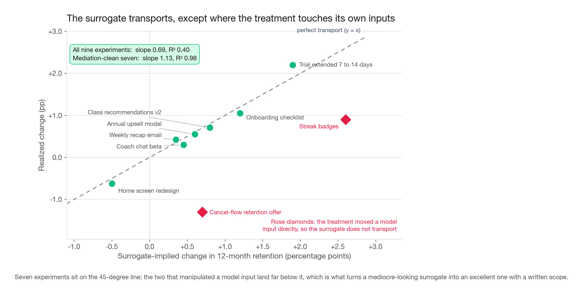
The only real evidence for transport is a library of past experiments with both readouts, what the surrogate said at week two and what the long-term metric did once it matured. If your company has run experiments for two years that library already exists and nobody has assembled it, which makes assembling it a great thing to propose in an interview. Here is Ridgeline's, nine tests, all in percentage points of twelve-month retention.
| Past experiment | Surrogate said | Truth turned out | Touches a model input directly |
|---|---|---|---|
| Onboarding checklist | +1.20 | +1.05 | no |
| Weekly recap email | +0.35 | +0.42 | no |
| Class recommendations v2 | +0.80 | +0.71 | no |
| Streak badges | +2.60 | +0.90 | yes, login days |
| Trial extended 7 to 14 days | +1.90 | +2.20 | no |
| Annual upsell modal | +0.60 | +0.55 | no |
| Cancel-flow retention offer | +0.70 | -1.30 | yes, week-1 cancels |
| Coach chat beta | +0.45 | +0.30 | no |
| Home screen redesign | -0.50 | -0.62 | no |
import numpy as np

pred = np.array([1.20, 0.35, 0.80, 2.60, 1.90, 0.60, 0.70, 0.45, -0.50])
real = np.array([1.05, 0.42, 0.71, 0.90, 2.20, 0.55, -1.30, 0.30, -0.62])
touches_input = np.array([0, 0, 0, 1, 0, 0, 1, 0, 0], dtype=bool)

def transport(p, r):
    A = np.vstack([p, np.ones_like(p)]).T
    b, *_ = np.linalg.lstsq(A, r, rcond=None)
    resid = r - A @ b
    r2 = 1 - (resid ** 2).sum() / ((r - r.mean()) ** 2).sum()
    return round(float(b[0]), 3), round(float(r2), 3)

print("all nine        slope, r2 =", transport(pred, real))
print("mediation-clean slope, r2 =", transport(pred[~touches_input],
                                               real[~touches_input]))
all nine slope, r2 = (0.694, 0.4)
mediation-clean slope, r2 = (1.131, 0.976)Across all nine the surrogate looks mediocre: slope 0.69, so it systematically overstates, with an R-squared of 0.40. A skeptical VP sees that and bans surrogate-based decisions. Drop the two experiments that violate condition two and the slope goes to 1.13 with an R-squared of 0.98. The surrogate is not mediocre, it is excellent inside a stated scope and invalid outside it, and the back-test is what let you draw the boundary instead of guessing.
That distinction is the whole argument. You are not claiming the surrogate is universally true. You are claiming it is accurate for changes working through general engagement, that nine data points support this, and that you have a written rule for the changes it does not cover.
How short a window can you get away with
Longer feature windows are more accurate and slower. Ridgeline measured the curve: a three-day window reaches AUC 0.66 with a transport slope of 0.71, seven days reaches 0.735 and slope 1.13, fourteen days 0.78 and 1.06, twenty-eight days 0.81 and 1.02. The AUC gain from fourteen to twenty-eight days is only 0.03 for two and a half extra weeks per experiment, and the slope is already near one at seven days, which matters more than AUC because a well-transporting surrogate with mediocre ranking still gives unbiased estimates, just noisier ones. The policy that falls out is seven days by default, twenty-eight for anything touching billing or cancellation, three days only as an automated safety trip.
Long-term holdbacks
A surrogate answers "will this change help in a year". A holdback answers a different and larger question: "is everything we shipped this year actually adding up".
What a holdback measures that no single experiment can
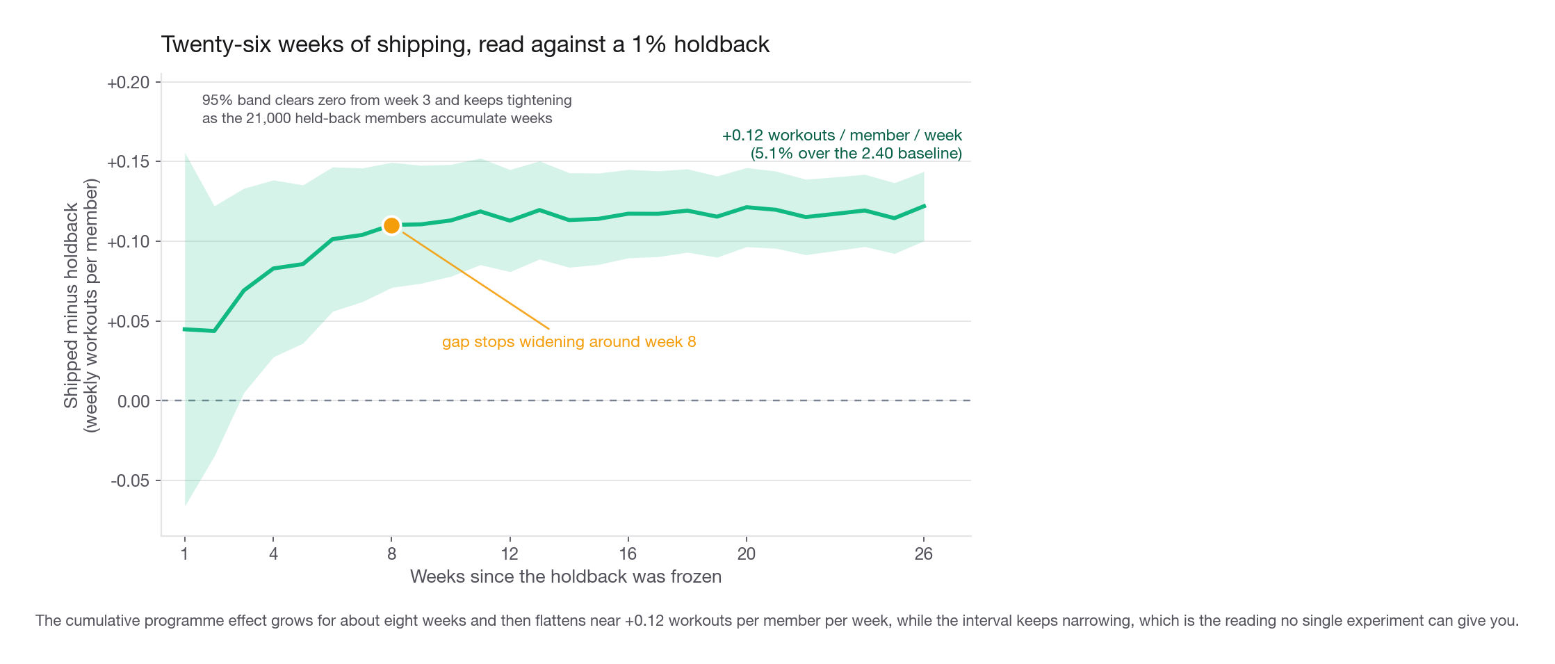
A holdback is a small slice of the population, chosen once, excluded from every launched change for a fixed period. After six months you compare it against everyone else and read the cumulative effect of the whole shipping programme.
This matters because experiment wins do not add. Ten experiments each measured at plus 0.4 percent do not give plus 4 percent: the wins overlap because they hit the same users by the same mechanism, some were false positives you shipped, some decayed with the novelty, and a few interact negatively. A holdback is the only instrument that reads the sum honestly. It is also the instrument for this lesson's problem, because if you suspect a benefit arrives late or a short-term win reverses, it lets you watch the gap over six months instead of two weeks.
The allocation arithmetic, which candidates get wrong
The variance of a difference in means depends on both arms and is dominated by the smaller one, which is what decides whether a holdback is worth having.
import numpy as np

TOTAL = 2_100_000
SIGMA, MEAN = 1.6, 2.4          # per-member 26-week average weekly workouts

for h in [0.50, 0.10, 0.05, 0.02, 0.01, 0.005]:
    n_hold = TOTAL * h
    n_ship = TOTAL - n_hold
    v = 1 / n_hold + 1 / n_ship
    n_eff = 4 / v               # balanced test with the same precision
    mde = 2.802 * SIGMA * np.sqrt(v)
    print(f"holdback {h*100:5.2f}%  n={n_hold:>9,.0f}  "
          f"equivalent balanced N={n_eff:>9,.0f}  "
          f"MDE={100*mde/MEAN:5.2f}% relative")
holdback 50.00% n=1,050,000 equivalent balanced N=2,100,000 MDE= 0.26% relative
holdback 10.00% n= 210,000 equivalent balanced N= 756,000 MDE= 0.43% relative
holdback 5.00% n= 105,000 equivalent balanced N= 399,000 MDE= 0.59% relative
holdback 2.00% n= 42,000 equivalent balanced N= 164,640 MDE= 0.92% relative
holdback 1.00% n= 21,000 equivalent balanced N= 83,160 MDE= 1.30% relative
holdback 0.50% n= 10,500 equivalent balanced N= 41,790 MDE= 1.83% relativeThe line to memorize: a one percent holdback out of 2.1 million has the precision of a balanced test with 83,000 users total, because the lopsided split threw away 96 percent of your effective sample. Moving from one percent to two doubles the withheld users and nearly doubles precision; moving from ten to fifty quintuples the withheld population to buy an MDE of 0.26 percent instead of 0.43. Each extra withheld user buys about 3.9 effective users on the one-to-two move, but only about 1.6 on the ten-to-fifty move. Precision is set by the smaller arm, so the first users you add to it are worth far more than the last.
Interview tip: If someone proposes a 0.1 percent holdback because it sounds cheap, compute its equivalent balanced sample size on the spot: it is almost always too small to detect anything actionable, which makes it pure cost.
The costs nobody puts in the deck
Engineering carry. Every launched change needs a permanent conditional so it can be suppressed for the holdback, and that code must survive six months of refactors. Teams routinely discover at week twenty that three of eleven shipped changes leaked in, which invalidates the comparison and cannot be reconstructed after the fact.
Member experience. You are deliberately giving 21,000 paying people a worse product for half a year. Say that internally rather than discovering it during a press cycle. The usual mitigation is rotation.
Rotation breaks the comparison you wanted. Rotate quarterly and you cannot measure a nine-month cumulative effect, because nobody was held back nine months. Pick one, long horizon with a fixed cohort or fair rotation with a short horizon, and saying that plainly marks someone who has run one.
Opportunity cost part one: the price of every extra week
The second half of the lesson is about money rather than measurement.
Ridgeline runs the onboarding redesign against 50 percent of new signups. Weekly signups are 22,000, so each arm gets 11,000 a week. After two weeks the treatment arm's surrogate score sits 2.1 points below control.
Is that real yet
Compute it rather than eyeballing it. The surrogate score has a standard deviation of about 0.197 here.
import numpy as np

SD_SCORE = 0.197
PER_ARM_PER_WEEK = 11_000

for weeks in [1, 2, 4]:
    n = PER_ARM_PER_WEEK * weeks
    se = SD_SCORE * np.sqrt(2 / n)
    print(f"{weeks} week(s): n={n:>6,} per arm, "
          f"SE={100*se:.3f}pp, 95% CI half-width={100*1.96*se:.3f}pp")
1 week(s): n=11,000 per arm, SE=0.266pp, 95% CI half-width=0.521pp
2 week(s): n=22,000 per arm, SE=0.188pp, 95% CI half-width=0.368pp
4 week(s): n=44,000 per arm, SE=0.133pp, 95% CI half-width=0.260ppAt two weeks the interval on that minus 2.1 points runs from about minus 2.47 to minus 1.73. No version of the truth has this change neutral. Continuing is not gathering evidence, it is paying for precision on a number you will not use.
What the extra week costs
A member who reaches twelve months is worth about 240 in downstream gross margin at Ridgeline, so a 2.1 point drop in predicted retention costs about 5.04 per signup in expectation. With 11,000 signups a week in the losing arm, that is 55,440 of expected lifetime value burned per additional week.
That is the number you bring to the room. Not "the test is losing", but "each further week costs roughly 55,000 in expected member value and buys a confidence interval we do not need". Nobody argues with the second sentence.
Write the futility rule before you start
Decide this before launch, because afterwards everyone is attached to the feature. The boundary is one line in the test plan: stop early and revert if, at any scheduled check after week one, the upper bound of the 95 percent interval on the surrogate delta sits below the minimum practical effect. Ridgeline's minimum practical effect for onboarding work is plus 0.5 points. At week two the upper bound is minus 1.73, so the rule fires and the decision is automatic.
A futility rule is not the same as stopping for a win. Peeking for a positive result inflates the false positive rate and needs a sequential correction. Stopping for futility is far more forgiving, because quitting early on a bad effect only risks abandoning something mildly good, and that error is cheap. Say that distinction out loud if an interviewer challenges you on peeking.
The mirror image: the cost of delaying a winner
Run it the other way. Had the redesign won by 1.4 points, 1.4 points times 240 is 3.36 per signup, and across 22,000 weekly signups over 52 weeks, 1,144,000 a year, full rollout is worth about 3.84 million a year. While the test keeps running at 50/50 the 11,000 a week sitting in control are the only ones missing out, so six extra weeks of confirmation forgoes about 222,000, priced on the same per-arm basis as the 55,440 a week a losing arm burns. Now the pressure runs toward shipping fast, and the right answer is a sequential design that can stop early on a win with the error rate controlled, rather than informal peeking or waiting out the calendar.
Interview tip: Whenever you recommend running longer, state the weekly cost of running longer in the same breath. Candidates who only ever recommend more data sound cautious; candidates who price the caution sound senior.
Opportunity cost part two: a significant win you refuse to ship
The question arrives as a paradox: the test won, the p-value is beautiful, why not ship. Three answers, and a complete response gives all three.
Answer one: significance is not size
The p-value answers whether the effect is distinguishable from zero. At 840,000 members per arm a genuinely tiny effect is comfortably distinguishable from zero, which is what power is for, and it means the p-value has stopped carrying information about whether anyone should care.
Ridgeline ran a class-ranking change at 840,000 per arm. Weekly workouts rose 0.31 percent relative, p equal to 0.004. Convert to money using the team's published elasticity, that a one percent lift in weekly workouts is worth 0.18 percent relative on twelve-month retention:
0.31 x 0.18 = 0.056 percent relative on retention.
Base retention 36.7 percent, so the absolute gain is 0.0205 points.
About 1.14 million members reach their first anniversary each year, 22,000 weekly signups over 52 weeks, so that is about 234 additional members retained per year.
At 240 each, roughly 56,000 per year.
Against that, the change needs a new ranking service: twelve engineer-months at a fully loaded 24,000 each is 288,000 to build, plus about 60,000 a year to keep alive. The carry alone exceeds the gain, so steady-state net is roughly negative 4,000 a year and the 288,000 build never pays back at all, before discounting and before accounting for what those three engineers would otherwise have done.
Watch which population the 240 applies to, because this is where the arithmetic goes wrong quietly. The onboarding redesign treats new signups, so its treated population and the first-anniversary population coincide. The class-ranking change touches all 2.1 million active members, but the metric and the 240 are both pinned to the twelve-month crossing, so only the cohort crossing it each year can be banked.
Do not ship, and notice the reason is arithmetic, not taste.
Answer two: complexity compounds
A new ranking service also means every future change to class ordering happens in two places, every incident review has one more suspect, and every new hire has one more thing to learn. That tax is small per change and charged on every change forever, so a change that adds a permanent branch to the codebase needs a bigger measured win than one that swaps a string.
Apply the rule symmetrically, or you are just being conservative. Had the same 0.31 percent lift come from reordering two rows on the home screen, one pull request adding no new surface, the cost side is near zero and the answer flips to ship immediately. Same effect size, same p-value, opposite decision. Effect size never decides on its own. The ratio of value to cost does.
Answer three: the change itself carries risk
Every deployment can break something, and a 56,000 per year gain does not survive one incident that takes checkout down for two hours. That is why the ship bar is higher on the payment path than on a settings screen.
The last row deserves its own habit: agree a minimum practical effect with the product owner before the test, in the same document as the sample size. Deciding what gain is worth having is not the data scientist's job. Refusing to run a test that cannot answer the question is.
Interview tip: If a prompt gives you a p-value but no effect size, ask for the effect size and the confidence interval before you answer. Interviewers include the omission on purpose.
When rerunning a test is legitimate
You lost a test eighteen months ago and someone wants to try again. Science or lobbying.
The default answer is no, and here is the arithmetic
If nothing changed, rerunning buys extra chances at a false positive. Three independent attempts at a 5 percent threshold give a 14.3 percent chance of at least one spurious win, and five give 22.6 percent. Nobody calls it multiple testing because the runs are years apart under different people, but the mathematics does not care about the calendar. The tell is the justification: "the team really believes in this one" is lobbying, a named change in the world is science.
Five reasons that qualify
| Reason to rerun | Evidence you should bring | Strength |
|---|---|---|
| Member mix has shifted | Segment shares then versus now, plus segment-level effects from the old test | Strong |
| A dependency shipped that the change needed | The dependency's own launch date and adoption | Strong |
| The old implementation was a weak version of the idea | Concrete diff, and ideally a qualitative reason the first build undersold it | Medium |
| The old test never resolved | Original confidence interval covering both zero and the effect you cared about | Strong |
| Seasonality or an external shock confounded it | The dates, and a comparable period without the shock | Medium |
| The team believes in it | none | None, do not run it |
The first row is the most common, so work it properly.
Reweighting an old test to today's population
An experiment never tells you which version is better in general, only which was better for the people in it. If the population has turned over, the old verdict describes a company that no longer exists. Ridgeline's 2024 test of a simplified home screen lost overall, but the effect was not uniform across usage segments, and the base has shifted heavily toward lighter users since.
| Usage segment | 2024 share | 2024 effect (percent relative) | Segment SE | 2026 share |
|---|---|---|---|---|
| Power, 4 or more workouts a week | 0.34 | -4.6 | 0.33 | 0.19 |
| Regular, 1 to 3 a week | 0.41 | +0.4 | 0.27 | 0.40 |
| Lapsing, under 1 a week | 0.25 | +3.4 | 0.48 | 0.41 |
import numpy as np

lift = np.array([-4.6, 0.4, 3.4])
se = np.array([0.33, 0.27, 0.48])
mix_2024 = np.array([0.34, 0.41, 0.25])
mix_2026 = np.array([0.19, 0.40, 0.41])

for label, w in [("as run, 2024 mix", mix_2024), ("reweighted, 2026 mix", mix_2026)]:
    est = (w * lift).sum()
    err = np.sqrt((w ** 2 * se ** 2).sum())
    print(f"{label:22s} {est:+.2f}%  95% CI "
          f"[{est - 1.96 * err:+.2f}, {est + 1.96 * err:+.2f}]")
as run, 2024 mix -0.55% 95% CI [-0.94, -0.16]
reweighted, 2026 mix +0.68% 95% CI [+0.22, +1.14]The test lost by 0.55 percent in 2024 and projects to a 0.68 percent win against today's mix. The mechanism is in the segment column: the design hurt power users badly, and power users have gone from a third of the base to a fifth while lapsing members went from a quarter to two fifths.
That number is a hypothesis, not a verdict
Here is where a good answer separates from a dangerous one. The reweighted interval excludes zero. It is still not a result. Three reasons you may not ship on it:
The segments were chosen after seeing the data. Nobody pre-registered a usage-tier breakdown. Slice an old test enough ways and some slice reverses the sign, because that is what noise does, and the reported interval does not price the search that found the segmentation.
Reweighting assumes segment effects are stable across two years. But the people inside "lapsing" in 2026 are not the people inside "lapsing" in 2024, precisely because acquisition changed. You are assuming the thing you claim has changed did not change in the way that matters.
You are asking old data a question it was not designed to answer. The test was powered for an overall effect, and the widest-error cell now carries the most weight.
So the output of a reweighting exercise is a prioritized rerun queue, not a decision. The defensible sentence is: "reweighting past losses to the current mix puts the simplified home screen top of the rerun queue, expected effect around plus 0.7 percent, and I want a fresh two-week test at 20 percent allocation to confirm."
Interview tip: The phrase to have ready is "re-analyzing an old test can generate a hypothesis but it cannot confirm one, because the question I am asking now is not the question the test was designed to answer."
The local optimum problem, which is the real lesson
If every decision is made by testing on the current member base, the product converges on whatever that base likes: early adopters, committed exercisers, people who already tolerated the rough edges. Three years of diligent experimentation can produce a product locally optimal for 2.1 million people that repels the next ten million. Every individual test was correct; the programme found a local maximum and camped there. Two mitigations, both structural rather than statistical:
Report segment effects on every test, especially for new and lapsed members, and treat a change that wins overall while losing among new members as a warning rather than a win.
Occasionally test on a population that is not your current one, for instance restricting a test to a market you are trying to grow into, and accept that it will be underpowered. An underpowered read of the population you want can beat a precise read of the population you have.
The written policy
All of it compresses into a one-page document agreed before the quarter starts. Describing this artifact in an interview makes you sound like someone who has run a programme, not a test.
What the whole answer sounds like in ninety seconds
Rehearse this shape for the subscription-retention prompt:
"Twelve-month retention is the outcome and I cannot run a fourteen-month test, so I need a short-window surrogate. I take members who joined more than thirteen months ago, use only their first seven days of behavior, and fit a model for whether they were still paying at month twelve. Ours gets an AUC around 0.74 and calibrates well by decile, so arm-level averages are meaningful. Before trusting it for this change I check two things: whether the new onboarding directly manipulates any feature in the model, because then it will over-read and I need the long readout instead, and how it back-tests against past experiments with both readouts, which for us means a slope near one for engagement changes and a bad overstatement for anything touching logins or the cancel flow. Then I run two weeks at fifty percent of new signups with a futility rule that reverts if the upper confidence bound sits below our minimum practical effect of plus half a point, because each week in a losing arm costs about 55,000 in expected member value. Separately I keep a one percent six-month holdback to check the year's changes add up, knowing it only has the precision of an 83,000-user balanced test and detects about 1.3 percent relative, nothing finer."
Nothing in that is a hedge. Every claim has a number behind it and every number has a decision attached.
Common traps
Proposing a proxy without saying how you validated it. The most common failure on this question. Fix: always name the mature cohort, the feature window, the held-out AUC, and the calibration check, in one sentence.
Validating only that the surrogate predicts. Prediction makes it a scoring tool. Fix: state the mediation condition and give the disqualifier, that a change acting directly on a model input invalidates the surrogate for that change.
Picking a proxy with a huge contrast on a tiny group. Week-one cancellation separates 4.8 percent from 39.5 percent retention and still has an AUC of 0.556. Fix: quote the population share alongside the contrast.
Treating a holdback as free because it is small. A 0.1 percent holdback costs real users and detects nothing. Fix: compute the equivalent balanced sample size and minimum detectable effect before agreeing an allocation.
Running a losing arm out of politeness. Fix: pre-register a futility boundary and price the weekly cost of continuing, so the conversation is arithmetic rather than anyone's feature.
Reading a p-value as a decision. At 840,000 per arm nearly everything is significant. Fix: convert the effect to annualized value, compare against build and carry cost, quote the payback period.
Applying the complexity argument only in one direction. If small effects always mean do not ship, you are not reasoning, you are being conservative. Fix: show the cheap-change counterexample where the same effect size flips the decision.
Shipping on a reweighted old result. The segmentation was chosen after the fact and the assumption of stable segment effects is exactly what is in question. Fix: state that the reweight generates the hypothesis and the fresh test confirms it.
Quick self-check
Answer these out loud, in full sentences.
Define a surrogate for annual subscription retention on a product of your choosing and state the two conditions it must satisfy. For the second, name a concrete change for which the surrogate would be invalid, and why.
A proxy separates 6 percent of users at 5 percent retention from the other 94 percent at 40 percent. Explain why that is excellent for targeting and poor for measuring an effect, and say what number makes the difference obvious.
A one percent holdback is proposed from a base of 4 million. Compute the equivalent balanced sample size, and say what it implies about the smallest detectable effect on a metric with mean 3.0 and standard deviation 2.0.
After two weeks a test is 1.8 points down on the surrogate with a 95 percent interval half-width of 0.3. State the futility rule you would have written before launch, whether it fires, and the two numbers that justify stopping.
A test wins by 0.4 percent relative with p equal to 0.002 at 900,000 per arm. Walk through the calculation that decides whether to ship, name every input, and give one version where you ship and one where you do not.
An old test lost by 0.5 percent and reweighting to today's mix projects a 0.7 percent win with an interval excluding zero. Give three reasons that cannot justify shipping, and write the sentence you would put in the rerun register instead.