1.2 Reading Regression Coefficients Like a Product Owner
Find the core decision, design, or behavior signal.
Turn the lesson into a concise response blueprint.
Name the trap you would avoid in a real interview.
Use these checkpoints as your reading path before diving into the full lesson.
- 1Why this matters in interviews
- 2The campaign we are going to interrogate
- 3Step zero: is the model worth interroga...
- 4Reference levels decide what the table...
- 5The default is alphabetical, and it is...
A fitted logistic regression hands you a table of numbers. Your job is not to read it out loud. It is to decide which rows are safe to turn into a roadmap item, which are artifacts of how you coded the data, and which are real but too small to be worth anybody's quarter. This lesson makes that call fast and defensible under pushback.
Why this matters in interviews
Coefficient reading is the cheapest probe of whether you understand a model or merely call .fit() on things. It takes twenty seconds to ask and separates candidates immediately. Three failure modes are what the interviewer listens for.
The first reads signs off the screen. "This market is positive, so it is good." Positive relative to what? If you cannot name the baseline in the same breath as the sign, you have read one column, not the model.
The second treats the largest absolute coefficient as the most important driver. That is a statement about units, not about the product. A coefficient on a variable ranging from 1 to 80,000 always looks tiny beside one on a zero/one flag, and neither tells you which moves the metric more.
The third says "significant" and stops. Significance tells you the sign is probably real, not that the effect justifies engineering time.
A strong answer moves through the table in a fixed order: what is the baseline, what is the direction, how big is the effect on a scale a human can picture, how confident are we in that size, and what would we ship.
Interview tip: Before you interpret a single coefficient out loud, say the reference level for every categorical in the model. It costs one sentence and it is the single clearest signal that you have done this before.
The campaign we are going to interrogate
Cadence is a fictional subscription audiobook app with roughly 320,000 active members. Lifecycle marketing sends each member one "Picked for you" push notification per week. The PM wants to raise the tap rate, the share of notifications that get a member back into the app within 24 hours. She does not want a model. She wants three things to change next sprint.
We pulled a 25 percent sample of one week of sends, 80,000 rows, one row per notification. The schema:
| Column | Type | Meaning |
|---|---|---|
notif_id | integer | Send counter, 1 to 80,000, in the order the queue drained. |
copy_length | category | brief or detailed body copy. |
greeting | category | named opens with the member's first name, generic does not. |
send_hour | integer | Local hour of send, 6 through 22. |
weekday | category | Day of send, Mon through Sun. |
market | category | US, UK, CA, AU, DE. |
titles_finished | integer | Lifetime audiobooks completed before this send. |
days_since_last_listen | integer | Recency at send time, in days. |
tapped | 0/1 | The label. Did the member open the app from it. |
This block regenerates the dataset behind every number here. It is deterministic, so your frame matches mine row for row, and it summarises to:
import numpy as np
import pandas as pd

SEED = 20260826
rng = np.random.default_rng(SEED)
N = 80_000

weekdays = np.array(["Mon", "Tue", "Wed", "Thu", "Fri", "Sat", "Sun"])
markets = np.array(["US", "UK", "CA", "AU", "DE"])

copy_length = rng.choice(["brief", "detailed"], N)
greeting = rng.choice(["named", "generic"], N)
send_hour = rng.integers(6, 23, N)
weekday = rng.choice(weekdays, N, p=[.16, .16, .16, .16, .14, .11, .11])
market = rng.choice(markets, N, p=[.46, .18, .14, .12, .10])
titles_finished = rng.poisson(3.1, N)
days_since_last_listen = rng.geometric(0.11, N) - 1

z = np.full(N, -3.85, dtype=float)
z += np.where(copy_length == "brief", 0.34, 0.0)
z += np.where(greeting == "named", 0.22, 0.0)
z += np.where(np.isin(weekday, ["Sat", "Sun"]), -0.47, 0.0)
z += 0.58 * np.exp(-((send_hour - 8.5) ** 2) / 5.5)      # commute peak
z += 0.71 * np.exp(-((send_hour - 20.0) ** 2) / 6.5)     # evening peak
z += np.select([market == "DE", market == "AU"], [-0.93, -0.14], 0.0)
z += 0.31 * np.log1p(titles_finished)
z += -0.028 * np.minimum(days_since_last_listen, 45)
z += 0.86 * ((market == "DE") & (copy_length == "detailed"))          # interaction
z += 0.52 * ((days_since_last_listen > 21) & (greeting == "named"))   # interaction

notifs = pd.DataFrame({
    "notif_id": np.arange(1, N + 1),
    "copy_length": copy_length,
    "greeting": greeting,
    "send_hour": send_hour,
    "weekday": weekday,
    "market": market,
    "titles_finished": titles_finished,
    "days_since_last_listen": days_since_last_listen,
    "tapped": rng.binomial(1, 1.0 / (1.0 + np.exp(-z))),
})
rows: 80000 taps: 3452 tap rate: 4.315%Three things in there bite the naive read later. send_hour has two humps, not one slope. titles_finished saturates. And two terms are interactions, so any coefficient assuming one number per feature averages over populations that behave differently.
Step zero: is the model worth interrogating at all
A coefficient table from a model that cannot predict is decoration. On these eight features the fit reaches an AUC of 0.606 against a 4.32% base rate, on 3,452 positives. That is unglamorous and normal for notification response, where most of the variance lives in whether the member was near their phone, and it is enough to interrogate. Had it come back at 0.51, say "I would not read these coefficients yet, the model has not found anything to read."
Note the positive count, not the row count: standard errors scale with the rare class, and 3,452 taps resolve a 10% odds change where 90 taps would not resolve 60%.
Reference levels decide what the table says
A categorical with k levels becomes k-1 indicator columns. The level without a column is the reference, and every remaining coefficient compares against it. This is the most misread part of a coefficient table, because the default reference is chosen for you and it is arbitrary.
The default is alphabetical, and it is almost never what you want
pandas.get_dummies(..., drop_first=True) sorts the levels and drops the first. See what that picks.
cats = ["copy_length", "greeting", "weekday", "market"]
print(notifs[cats].apply(lambda s: sorted(s.unique())[0]))
copy_length brief
greeting generic
weekday Fri
market AU
dtype: objectThe alphabet handed us brief, generic, Fri and AU, an incoherent set: brief is the variant marketing wants to roll out, generic the one they want to retire, AU the second-smallest market. Fit it that way and see what the table seems to say.
import statsmodels.api as sm

NUMERIC = ["notif_id", "send_hour", "titles_finished", "days_since_last_listen"]
dummies = pd.get_dummies(notifs[cats], drop_first=True).astype(float)
X_default = pd.concat([pd.Series(1.0, index=notifs.index, name="intercept"),
                       notifs[NUMERIC].astype(float), dummies], axis=1)
default_fit = sm.Logit(notifs["tapped"], X_default).fit(disp=0)
print(default_fit.params.sort_values(ascending=False).round(4))
greeting_named 0.2529
market_UK 0.2326
market_US 0.1727
market_CA 0.1618
weekday_Mon 0.0689
titles_finished 0.0662
send_hour 0.0149
notif_id 0.0000
weekday_Tue -0.0115
weekday_Thu -0.0175
weekday_Wed -0.0196
days_since_last_listen -0.0210
market_DE -0.2883
copy_length_detailed -0.3300
weekday_Sat -0.3389
weekday_Sun -0.5477
intercept -3.4205Two readings a hurried analyst produces, both wrong in the way that matters. The first is "Tuesday, Wednesday and Thursday hurt us." All three carry negative coefficients, and all three have tap rates above the campaign average, Wednesday at 4.57% against a 4.32% base. Negative here means "below Friday", not "below average", and not "bad". Friday outranks all three midweek days and loses only to Monday, so it pulls the whole block under zero.
The second is that two winning changes appear with opposite signs: short copy wins as copy_length_detailed at -0.33, personalization as greeting_named at +0.25. Half the table is phrased as the cost of what you would retire and half as the gain from what you would ship, purely because of how level names sort.
A block of negative coefficients never means the categorical is a liability. It means every level in it is weaker than the one you left out.
Setting the reference on purpose
Pick the reference so the table answers the question you were asked. Three rules cover most cases.
Current default, when the question is "should we change". Cadence's live template is detailed copy with a generic greeting, so those baselines turn every coefficient into the value of switching.
Largest cell, when the question is "where do we grow". The US is 46% of sends, so
USasks how far each market sits from the one carrying half our volume.The level under review, when the question is "should we stop". Marketing wants to kill the weekend slot, so
Satprices the move.
The same model, with references chosen for those questions.
REFS = {"copy_length": "detailed", "greeting": "generic",
        "weekday": "Sat", "market": "US"}

def design(frame, refs, numeric):
    X = pd.DataFrame({"intercept": np.ones(len(frame))}, index=frame.index)
    for col in numeric:
        X[col] = frame[col].astype(float)
    for col, ref in refs.items():
        for level in sorted(frame[col].unique()):
            if level != ref:
                X[f"{col}_{level}"] = (frame[col] == level).astype(float)
    return X

X = design(notifs, REFS, NUMERIC)
fitted = sm.Logit(notifs["tapped"], X).fit(disp=0)
table = pd.DataFrame({"coef": fitted.params, "se": fitted.bse,
                      "p": fitted.pvalues})
table["odds_ratio"] = np.exp(table["coef"])
print(table.sort_values("coef", ascending=False).round(4))
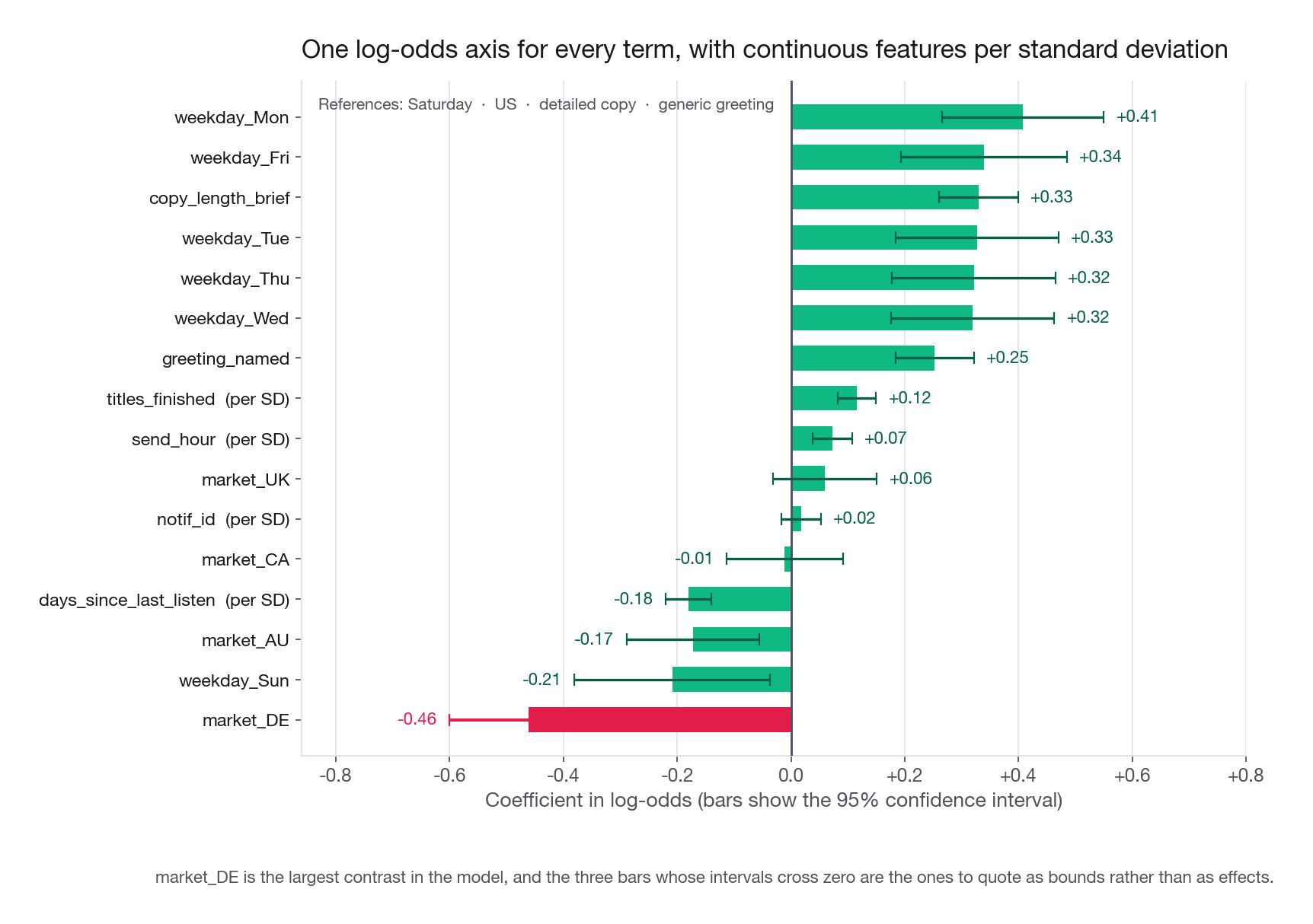
That is the table the rest of this lesson reads. Weekdays compare against Saturday, markets against the US, copy against detailed, greeting against generic.
| Term | Coefficient | Std error | p value | Odds ratio |
|---|---|---|---|---|
| weekday_Mon | 0.4078 | 0.0723 | 1.7e-08 | 1.50 |
| weekday_Fri | 0.3389 | 0.0745 | 5.5e-06 | 1.40 |
| copy_length_brief | 0.3300 | 0.0353 | 8.5e-21 | 1.39 |
| weekday_Tue | 0.3273 | 0.0730 | 7.3e-06 | 1.39 |
| weekday_Thu | 0.3214 | 0.0733 | 1.2e-05 | 1.38 |
| weekday_Wed | 0.3193 | 0.0733 | 1.3e-05 | 1.38 |
| greeting_named | 0.2529 | 0.0351 | 6.2e-13 | 1.29 |
| titles_finished | 0.0662 | 0.0097 | 8.5e-12 | 1.07 |
| market_UK | 0.0598 | 0.0466 | 0.199 | 1.06 |
| send_hour | 0.0149 | 0.0036 | 3.1e-05 | 1.02 |
| notif_id | 0.00000077 | 0.00000076 | 0.311 | 1.00 |
| market_CA | -0.0109 | 0.0522 | 0.835 | 0.99 |
| days_since_last_listen | -0.0210 | 0.0024 | 1.1e-18 | 0.98 |
| market_AU | -0.1727 | 0.0594 | 0.0036 | 0.84 |
| weekday_Sun | -0.2088 | 0.0877 | 0.017 | 0.81 |
| market_DE | -0.4611 | 0.0709 | 7.9e-11 | 0.63 |
| intercept | -3.9167 | 0.0975 | 0.000 | 0.02 |
Same model, same data, same likelihood, a completely different first read. The weekday block is now clean: five weekdays cluster between 0.32 and 0.41 above Saturday, Sunday sits 0.21 below. Both copy_length_brief and greeting_named are positive, so both read as gains, which is what the PM buys.
The contrast you want may not be in the table
Every categorical coefficient compares against the reference and nothing else. The table says Monday beats Saturday and Wednesday beats Saturday. It does not say whether Monday beats Wednesday.
Two ways to get it: refit with Wed as the reference, or run a linear hypothesis test on the existing fit. Refit and Monday returns 0.0885, standard error 0.0591, an odds ratio of 1.09 with a 95% interval of 0.97 to 1.23 and p equal to 0.13. The weekdays are indistinguishable and the whole weekday signal is "not the weekend". Do not move everything to Monday, move the weekend slot onto weekdays, and mean both days when you say it. Sunday taps at 2.76% and Saturday at 3.37%, against 4.56% to 4.96% Monday through Friday. Saturday's weakness is the easiest thing on this page to miss, because Saturday is the reference: its penalty is folded into the intercept and there is no weekday_Sat row to read. The five weekday coefficients of 0.32 to 0.41 are Saturday's penalty stated backwards, and the probability table below prices the Saturday half of that move at about plus 2.0 points on the 4.3% base. An analyst who reads only the rows that exist ships a Sunday fix and leaves 8,677 sample-week sends parked in the second-worst slot on the calendar.
The same trick sizes Germany: refit with DE as the market reference and the UK returns 0.5209, an odds ratio of 1.68. Germany runs at roughly 60% of the odds of the English-language markets, and that has a cause you can act on.
Interview tip: When an interviewer asks whether two non-reference levels differ, do not eyeball the gap between their coefficients, because the two share a covariance and the difference of their standard errors is not the standard error of their difference.
Three scales, and knowing which one your audience thinks in
A logistic regression is linear in log-odds, multiplicative in odds, curved in probability. Mixing those views up is the most common way a good analysis gets miscommunicated.
| Scale | What a coefficient of 0.330 means | Who thinks in it |
|---|---|---|
| Log-odds | Adds 0.330 to the linear predictor, whatever the other features do | The model, nobody else |
| Odds ratio | Multiplies the odds of a tap by exp(0.330) = 1.39 | Analysts, risk people |
| Probability | Depends where you start: 0.8 points at a 2.1% base, 3.7 at an 11% base | PMs, execs, budget holders |
Log-odds is where the additivity lives, which is why the model works there, and nobody approved a project because the log-odds went up.
Exponentiating gives a clean multiplicative statement: brief copy raises tap odds by about 39%. People hear "raises the tap rate by 39%", and the two coincide only when the base rate is tiny. At our 4.3% average an odds ratio of 1.39 lands at 5.90%, a 1.37x lift; at 40% it lands at 48.1%, a 1.20x lift.
Probability is what gets funded, so compute it at a stated base rate
Translate on the spot, and say which base rate you used. Cadence has three segments worth naming: lapsed members on generic copy tap at about 2.1%, the campaign averages 4.3%, and the best-responding profile we can build, recent listeners in an English-language market on brief personalized copy in the evening, taps near 11%.
def prob_delta(base_p, coef):
    base_odds = base_p / (1 - base_p)
    new_odds = base_odds * np.exp(coef)
    return 100 * (new_odds / (1 + new_odds) - base_p)

for base in [0.021, 0.043, 0.11]:
    print(base,
          round(prob_delta(base, 0.3300), 2),    # brief copy
          round(prob_delta(base, 0.2529), 2),    # named greeting
          round(prob_delta(base, 0.4078), 2),    # Monday vs Saturday
          round(prob_delta(base, 0.0662), 2))    # one extra finished title
0.021 0.8 0.59 1.02 0.14
0.043 1.58 1.17 2.03 0.28
0.11 3.67 2.73 4.67 0.67| Change | At a 2.1% lapsed base | At the 4.3% campaign base | At an 11% best-case base |
|---|---|---|---|
| Brief copy instead of detailed | +0.80 pts | +1.58 pts | +3.67 pts |
| Named greeting instead of generic | +0.59 pts | +1.17 pts | +2.73 pts |
| Monday instead of Saturday | +1.02 pts | +2.03 pts | +4.67 pts |
| One extra finished title | +0.14 pts | +0.28 pts | +0.67 pts |
One coefficient produces a four-and-a-half-fold range of impact depending on the segment. When a PM asks how much this moves the number, answer "for which segment".
Interview tip: Translate log-odds into percentage points at a named base rate, and say the base rate out loud, because "about plus 1.6 points on our 4.3% weekly average" lands where "it raises the log-odds by 0.33" does not.
The number a PM can actually budget against
For a business case, score the counterfactual: take the real population, flip the field you would ship, sum the predictions.
def expected_taps(frame_X, params, **overrides):
    Z = frame_X.copy()
    for col, value in overrides.items():
        Z[col] = value
    scores = 1 / (1 + np.exp(-(Z.values @ params.values)))
    return float(scores.sum())

base_taps = expected_taps(X, fitted.params)
all_brief = expected_taps(X, fitted.params, copy_length_brief=1.0)
all_named = expected_taps(X, fitted.params, greeting_named=1.0)
both = expected_taps(X, fitted.params, copy_length_brief=1.0, greeting_named=1.0)
print(round(base_taps), round(all_brief), round(all_named), round(both))
3452 3991 3865 4465Brief copy everywhere is worth about 539 extra taps in this 80,000-row sample, a 15.6% lift, roughly 2,150 a week across the full base. A named greeting everywhere is worth about 413, a 12.0% lift.
Two warnings. First, observational coefficients are not causal estimates, and copy length was not randomised here. Say so, and say the fix: a two-arm test, brief against detailed, with copy length as the only difference. Size it off the arm rates, not off the rollout lift, because those are two different contrasts and mixing them is a common way to over-order sample. The 15.6% is what moving the whole population off today's 50/50 mix buys. The test compares one arm against the other, and scoring both arms gives 3.64% for detailed against 4.99% for brief, a 37% relative effect, which at 80% power and a two-sided alpha of 0.05 needs roughly 3,600 sends per arm. Feed the model 4.3% and 15.6% instead and it asks for 15,400 per arm, more than four times the sends, on a test that is not the one you described. The rule is that the base rate in a power calculation is the control arm's rate, not the campaign's pooled rate. Second, the stacked figure of 4,465 is a 29.3% lift and you should refuse to quote it, because stacking assumes independence and that nobody reacts to being messaged better.
Magnitude is not importance until you fix the scale
Rank the continuous features by absolute coefficient and you get titles_finished at 0.066, days_since_last_listen at 0.021, send_hour at 0.015, and notif_id at 0.00000077. That is not an importance ranking, it is a ranking of how the columns were measured: notif_id spans 80,000 units, recency 92 days, completions 15, while the indicators already cover their whole range.
Standardizing puts continuous features on one axis
Rescale each continuous variable to mean zero and unit standard deviation before fitting, so its coefficient reads as the effect of a one standard deviation move.
X_std = X.copy()
for col in NUMERIC:
    X_std[col] = (X_std[col] - X_std[col].mean()) / X_std[col].std(ddof=0)

std_fit = sm.Logit(notifs["tapped"], X_std).fit(disp=0)
print(std_fit.params[NUMERIC].round(4))
print(X[NUMERIC].std(ddof=0).round(3))
notif_id 0.0177
send_hour 0.0728
titles_finished 0.1160
days_since_last_listen -0.1795
notif_id 23094.011
send_hour 4.880
titles_finished 1.754
days_since_last_listen 8.539| Feature | Raw coefficient | Std deviation | Per-SD coefficient | Per-SD odds ratio |
|---|---|---|---|---|
days_since_last_listen | -0.0210 | 8.54 days | -0.180 | 0.84 |
titles_finished | 0.0662 | 1.75 titles | 0.116 | 1.12 |
send_hour | 0.0149 | 4.88 hours | 0.073 | 1.08 |
notif_id | 0.00000077 | 23,094 sends | 0.018 | 1.02 |
The ranking reorganises. Recency was second by raw coefficient and is first on a common axis: one standard deviation of staleness, about 8.5 days, costs roughly 16% of the tap odds. Completions drop to second.
notif_id is worth pausing on, because standardizing separates the two reasons a raw coefficient can be tiny. A tiny coefficient on a wide-ranging feature can hide a large effect. Here it does not: per standard deviation it is 0.018, with a 95% odds-ratio interval of 0.98 to 1.05. Queue position is genuinely null, which is the answer you want, since a real effect there would mean send order is leaking into response.
The catch is presentational. Nobody knows what a standard deviation of staleness is, so standardize to rank drivers for yourself, then translate back into business units to present.
A version that presents better is the plausible swing: multiply each coefficient by a range the business could realise. Pulling a member from 21 days stale to 7 is 14 times 0.021, about 0.29 in log-odds, comparable to the named greeting. That also separates levers from context. Market is among the largest coefficients on the board and is not a lever, because you cannot move a member to the UK. State that distinction, because it turns a read into a recommendation.
What the intercept is for
The intercept is -3.917, a predicted tap probability of 1.95% for a US member on detailed generic copy, on a Saturday, at hour zero, with zero finished titles, zero days since last listen and a notif_id of zero. That row cannot exist: sends run 06:00 to 22:00 and notif_id starts at 1.
Do not read the intercept as a baseline rate. Use it for headroom only. The controllable coefficients sum to about 0.99 against a -3.92 intercept, so the levers can move the outcome. If it were -30 with the same coefficients, no template tweak would matter and the honest recommendation would be to find a different problem.
What a p-value buys you and what it does not
Significance says whether a sign is distinguishable from zero, not whether it matters. Four readings you should produce on demand:
Significant and large.
copy_length_briefat 0.330, p near 1e-20. Ship a test.Significant and small.
send_hourat 0.0149, p equal to 3.1e-05. Real, tiny, and describing the wrong shape entirely.Not significant, tight interval.
market_CAat -0.011, p equal to 0.835, odds ratio interval 0.89 to 1.10. Canada is at parity with the US to within about 10%.Not significant, and that is the finding.
notif_idat p equal to 0.311. Queue position does not predict response, which rules out a class of delivery bug.
The last two are where candidates stop early. "Not significant, ignore it" is weaker than "the interval rules out anything worse than an 11% odds penalty, so Canada and the US are one market for planning". A null tells you where the story is not. The story is that Germany runs at about 63% of US odds and Australia at 84%, and Germany is far enough out to chase.
Interview tip: Always convert a non-significant coefficient into a confidence interval before dismissing it, because "we can rule out an effect larger than X" is a finding and "it was not significant" is a shrug.
The coefficient that averages two opposite stories
Germany is the most interesting row in the table and the main-effects model cannot explain it. Before reaching for a story about localisation or pricing, cross the market against the levers you have. One line.
print(notifs.pivot_table(index="market", columns="copy_length",
                         values="tapped", aggfunc="mean").round(4))
copy_length brief detailed
market
AU 0.0448 0.0319
CA 0.0538 0.0359
DE 0.0210 0.0367
UK 0.0538 0.0420
US 0.0548 0.0356Look at the DE row. Everywhere else brief beats detailed by 1.2 to 1.9 percentage points. In Germany it reverses: brief taps at 2.10%, detailed at 3.67%. The copy_length_brief coefficient of 0.330 is not a fact about Cadence members. It is an average over four markets where brief wins and one where it loses badly, dominated by the US at 46% of sends.
A regression finds this, but only if you ask. Add the interaction term explicitly.
X_int = X.copy()
X_int["DE_x_brief"] = ((notifs["market"] == "DE") &
                       (notifs["copy_length"] == "brief")).astype(float)
int_fit = sm.Logit(notifs["tapped"], X_int).fit(disp=0)
for term in ["copy_length_brief", "market_DE", "DE_x_brief"]:
    print(term, round(int_fit.params[term], 4), round(int_fit.bse[term], 4),
          f"{int_fit.pvalues[term]:.2g}")
print("net brief in DE:",
      round(int_fit.params["copy_length_brief"] + int_fit.params["DE_x_brief"], 4))
print("LR chi2 vs main effects:", round(2 * (int_fit.llf - fitted.llf), 2))
copy_length_brief 0.3982 0.0368 2.5e-27
market_DE 0.0014 0.0894 0.99
DE_x_brief -0.9774 0.1429 8.1e-12
net brief in DE: -0.5792
LR chi2 vs main effects: 49.07That rewrites two rows at once. The brief-copy effect outside Germany is larger than the main-effects model said, 0.398 rather than 0.330, an odds ratio of 1.49. Inside Germany the net effect is -0.579, an odds ratio of 0.56, so brief copy costs Germany nearly half its tap odds. And market_DE collapses to 0.0014 at p equal to 0.99: once copy length may behave differently there, no market penalty is left to explain. The "weak market" finding was a copy problem in a geography costume, and a likelihood ratio test on one degree of freedom gives a chi-squared of 49.1.
Score the two rollouts against the interaction model.
de_flag = (notifs["market"] == "DE").astype(float)
brief_all = expected_taps(X_int, int_fit.params,
                          copy_length_brief=1.0, DE_x_brief=de_flag)
brief_not_de = expected_taps(X_int, int_fit.params,
                             copy_length_brief=1.0 - de_flag, DE_x_brief=0.0)
print(round(brief_all), round(brief_not_de))
3990 4118A blanket brief rollout gains about 538 taps. Keeping detailed copy in Germany gains about 666, roughly 24% more, from a carve-out affecting 10% of sends. That gap of 128 taps a week is why interactions are worth checking before you present a main-effects table.
The greeting has the same structure. Among members more than 21 days lapsed a named greeting takes the tap rate from 2.15% to 4.22%; among active members it moves 3.94% to 4.88%. Fit that interaction and the named coefficient among lapsed members is 0.700, an odds ratio of 2.01, against 0.227 for everyone else. Personalization is a reactivation tactic averaged into a mild global one.
Interview tip: When one level of a categorical is an outlier, cross it against your controllable features before you invent a market-level explanation, because a reversal inside one segment is far more common than a genuine geography effect.
When two columns tell the same story
Cadence's feature table ships titles_finished raw, and the analyst who noticed the saturating shape added a log version beside it rather than replacing it. The two correlate at 0.95, which wrecks the coefficient table.
X_both = X.copy()
X_both["log_titles"] = np.log1p(notifs["titles_finished"]).astype(float)
both_fit = sm.Logit(notifs["tapped"], X_both).fit(disp=0)
cols = ["titles_finished", "log_titles"]
print(both_fit.params[cols].round(5))
print(both_fit.bse[cols].round(5))
titles_finished -0.02092
log_titles 0.34879
titles_finished 0.03320
log_titles 0.12722The raw column flipped sign. Alone it was +0.066, standard error 0.0097, p near 1e-11. Beside its own logarithm it is -0.021 with a standard error of 0.0332, a 3.4x inflation, and a p value of 0.53. The variance inflation factor for both columns is 10.6.
The model still predicts fine: log-likelihood barely moves, from -13998.3 with the raw column alone to -13994.4 with both. Collinearity damages attribution, not prediction, and attribution is the point of a coefficient table. The joint effect of "how much this member listens" is estimated accurately; its split between two columns is nearly arbitrary, and the standard errors say so. Drop to a single-segment sample and it stops behaving at all.
rng2 = np.random.default_rng(7)
for n in [4_000, 12_000, 40_000]:
    idx = rng2.choice(len(notifs), n, replace=False)
    sub = sm.Logit(notifs["tapped"].iloc[idx], X_both.iloc[idx]).fit(disp=0)
    print(n, round(sub.params["titles_finished"], 4),
          round(sub.params["log_titles"], 4))
4000 -0.1843 1.1575
12000 0.1517 -0.4186
40000 -0.0551 0.4375Three subsamples, three stories. At 12,000 rows the log column returns -0.42, which reads as "finishing more audiobooks makes members less likely to tap". Present that and you have manufactured a false insight out of a redundancy in your feature table.
| Symptom | What it looks like | What it is not |
|---|---|---|
| Standard errors 3x to 10x too large | Wide intervals, borderline p values on features you know matter | A weak feature |
| Sign flips when you add or drop a column | Two columns splitting one effect | A discovered interaction |
| Large individual p values, jointly significant pair | Redundant encoding of one behaviour | Evidence the behaviour does not matter |
The fix is not a statistical trick. Decide which encoding answers the product question and keep exactly one. The log version wins here: alone it gives 0.272 with a standard error of 0.038 and a log-likelihood of -13994.6, better than the raw column and within noise of using both. If you genuinely need two listening features, use lifetime completions plus recent completions as a share of lifetime, which measures momentum rather than repeating volume.
The linearity trap
A continuous feature enters a logistic regression as a straight line in log-odds. That is a strong assumption, and wrong for most behavioural variables, which peak in the middle of their range or, worse, twice.
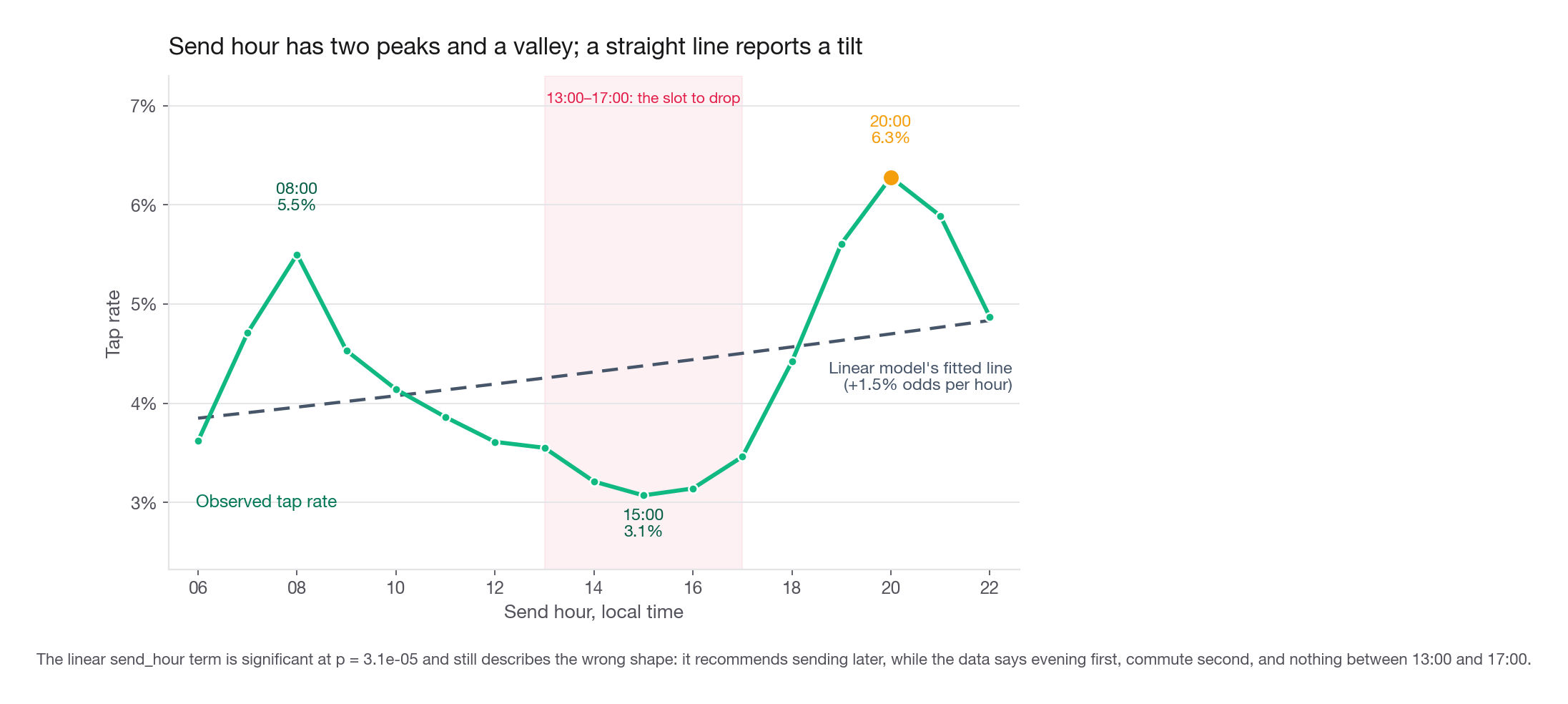
send_hour is the clean example. Its coefficient is 0.0149 at p equal to 3.1e-05, so it passes every test a careless reader applies, and it says each later hour raises tap odds by about 1.5%, which recommends sending as late as the queue allows. The truth has nothing to do with a slope. Bin the hour and look.
slots = pd.cut(notifs["send_hour"], [5, 9, 13, 17, 21, 22],
               labels=["commute_6_9", "midday_10_13", "afternoon_14_17",
                       "evening_18_21", "late_22"])
print(notifs.groupby(slots, observed=True)["tapped"]
      .agg(["size", "mean"]).round(4))
size mean
send_hour
commute_6_9 18760 0.0459
midday_10_13 18950 0.0379
afternoon_14_17 18994 0.0322
evening_18_21 18695 0.0555
late_22 4601 0.0487Two peaks and a valley. The commute window runs at 4.59%, the day sags to 3.22% by mid-afternoon, and evening is the best slot at 5.55%. Hour by hour it is sharper: 08:00 taps at 5.50%, 15:00 at 3.07%, 20:00 at 6.28%, more than double the trough. A straight line cannot express "up, down, up", so it fits a shallow tilt that describes none of the three regions.
Replace the raw hour with slot indicators and the fit tells the truth.
X_slots = X.drop(columns=["send_hour"]).copy()
for level in ["midday_10_13", "afternoon_14_17", "evening_18_21", "late_22"]:
    X_slots[f"slot_{level}"] = (slots == level).astype(float)

slot_fit = sm.Logit(notifs["tapped"], X_slots).fit(disp=0)
print(slot_fit.params.filter(like="slot_").round(4))
print(slot_fit.pvalues.filter(like="slot_").round(4))
slot_midday_10_13 -0.2004
slot_afternoon_14_17 -0.3706
slot_evening_18_21 0.1972
slot_late_22 0.0565
slot_midday_10_13 0.0001
slot_afternoon_14_17 0.0000
slot_evening_18_21 0.0000
slot_late_22 0.4637With the commute window as reference, midday costs 0.20, afternoon 0.37, and evening gains 0.20. Best to worst slot is 0.57 in log-odds, an odds ratio of 1.77, larger than the copy lever and about the size of the German copy problem. The linear term reported 1.5% per hour and threw all of that away, and AUC moves from 0.606 to 0.619.
The read-out changes completely. The linear model said "send later". The binned model says "evening first, commute second, never 13:00 to 17:00", which anyone can implement.
Interview tip: If an interviewer hands you a coefficient table with a continuous variable in it, ask whether the relationship was checked for monotonicity before you interpret the sign, because naming the assumption before you are asked about it is worth more than any single interpretation.
Two related shapes: saturation, which titles_finished shows past about six completions, and thresholds, which days_since_last_listen shows near three weeks. Both are invisible in a coefficient and obvious in a five-bucket table.
From coefficient table to product read-out
The table is an input. The output is a short list of changes with sizes attached.
A weak read-out: "Weekday is the biggest driver at around 0.4. Germany is significantly negative. Brief copy is significant with a very low p value. Later hours are better. Send brief personalized notifications on Monday evening and investigate Germany."
A strong read-out: "Three of the eight features are levers, the rest are context, and I am ranking the levers on counterfactual volume inside one shared model rather than on coefficient size, so the ordering survives the fact that these features are on different scales. The largest lever is send time, but not as the coefficient suggests: the linear term says 1.5% odds per hour while the real shape has two peaks, 08:00 at 5.5% and 20:00 at 6.3%, with a 3.1% trough at 15:00. Best to worst slot is 0.57 in log-odds, an odds ratio of 1.77. Moving every send into the evening window scores about 970 extra taps on this 80,000-row sample, roughly 3,900 a week across the full base. The version I would actually ship is narrower, stop sending between 13:00 and 17:00 and push that quarter of the volume into the evening, and it scores about 440, roughly 1,750 a week. Second is copy length: brief raises tap odds about 39%, which is 1.6 points on our 4.3% weekly average. I would not flip the whole channel, because the effect reverses in Germany, where brief taps at 2.1% against 3.7% for detailed. Fit that interaction and the German market penalty disappears, from an odds ratio of 0.63 to nothing. Germany was never a weak market, it is a broken template, and the carve-out scores about 660 against about 535 for the blanket rollout, roughly a quarter more from a rule that touches 10% of sends. Third is the greeting, about 29% in odds overall but really a reactivation tactic: among members over 21 days lapsed it doubles the tap rate, 2.1% to 4.2%. On context, weekday matters only as a weekend penalty, and Monday versus Wednesday has a p value of 0.13, so I would move the whole weekend slot onto weekdays rather than chase Monday, and I mean both days: Saturday taps at 3.4% and Sunday at 2.8% against 4.6% to 5.0% Monday through Friday. Saturday is the reference in this fit, so its penalty never appears as a row at all, it appears as the five positive weekday coefficients. Queue position is null at p equal to 0.31, ruling out a delivery-order bug. All of this is observational, so each item is a test to run rather than a change to make, and I would order the tests by cost rather than by size: the afternoon-against-evening slot test first at roughly 1,200 sends per arm, then the German copy carve-out at roughly 1,800, then the campaign-wide copy test at roughly 3,600. The slot test happens to be both the biggest lever and the cheapest test, which is the easiest sequencing argument I will ever get to make."
The second answer is longer because every claim carries a size, a scale and a caveat, and separates what the model found from what it can support.
Common traps
Reading a sign without naming the reference. Print the dropped level for every categorical and put it in your first sentence. Three midweek days here carry negative coefficients while sitting above the campaign average, purely because Friday was baseline. The subtler half of this trap is that the reference never gets a row of its own, so its weakness is easy to leave unfixed: Saturday taps at 3.37% and is the second-worst day on the calendar, and nothing in the coefficient table says so. Print the baseline's observed rate next to the coefficients or you will ship an action for every level except the one you are comparing against.
Letting the alphabet choose your baselines. Set references to the current production configuration so every coefficient reads as the value of a change, rather than half as costs and half as gains.
Ranking importance by raw coefficient size. Units are arbitrary. Standardize to rank, or multiply by a plausible business range, then translate back to present.
Treating a low p value as a green light. Ask for the effect in percentage points first. The
send_hourterm is significant at 3e-05 and describes the data wrongly.Dismissing a null coefficient without an interval. "Canada is within 10% of the US either way" is information. "Not significant" is not.
Accepting a market-level story before checking segments. Germany looked like a 37% odds penalty and was entirely a copy-length reversal. Cross outlier levels against your levers before writing "localisation" in a deck.
Assuming a continuous effect is monotone. Send hour has two peaks. A straight line reported a 1.5% per hour tilt and hid an odds ratio of 1.77 between best and worst slot.
Leaving two encodings of one behaviour in the model. Raw and log completions split one effect, inflate standard errors 3.4x, and flip signs from one subsample to the next. Keep one.
Quoting a stacked counterfactual. Adding coefficients and exponentiating assumes independence and no member reaction. Label the combined 29% an upper bound, and say "associated with" rather than "causes" until an experiment you have named and sized says otherwise.
Quick self-check
Answer these out loud, in full sentences, the way you would in a live interview.
In the alphabetical fit
weekday_Wedcame back at -0.0196, yet Wednesday's observed tap rate is 4.57% against a 4.32% average. Explain to a PM in two sentences how both are true.A colleague reports an odds ratio of 1.39 on brief copy and tells the room it lifts taps by 39%. Give a base rate where that is roughly right and one where it is badly wrong.
titles_finishedhas a raw coefficient of 0.066 andnotif_idone of 0.00000077. Give two reasons the second could still be the bigger driver, say what settles it, and what that computation showed here.market_CAcame back at -0.011 with a p value of 0.835. Write the summary-deck sentence, containing a bound rather than the word "insignificant".The main-effects model put Germany at an odds ratio of 0.63 and the interaction model puts it at 1.00. Name what changed, the one-line check that would have caught it before fitting, and what you would ship differently.
The linear
send_hourcoefficient is significant at p near 3e-05. Explain why you would still refuse to recommend later send times, and name the diagnostic you would run first.