3.1 Personalization: From Segments to Individuals
Find the core decision, design, or behavior signal.
Turn the lesson into a concise response blueprint.
Name the trap you would avoid in a real interview.
Use these checkpoints as your reading path before diving into the full lesson.
- 1Why this matters in interviews
- 2The three levels of a decision rule
- 3Why personalization pays, and the argum...
- 4The famous argument: nobody is average
- 5The argument that actually holds: the g...
An interviewer says: "We send one weekly nudge to everybody. Should we personalize it?" The wrong reflex is to say yes and start describing a recommender. The right reflex is to work out three numbers first: what you gain by fixing the single global rule, what you gain on top of that by letting the rule vary per user, and how many weeks of traffic it takes to prove the second number is real. Very often the first is large and cheap and the second is small and expensive. This lesson teaches you to compute both and to know when the honest recommendation is not to personalize at all.
Why this matters in interviews
Earlier in this course you pulled insights out of models: which levers move the outcome, which segments differ, what shape a variable has. Every one of those answers is a statement about an average. "Short copy beats long copy" means short copy wins when you pool everyone. Personalization is the question that comes right after: does short copy win for this user, and if not, who gets the long version?
A weak answer sounds like: "I'd build a model to predict engagement per user and show them the content with the highest predicted engagement." That describes a content ranker, not a decision rule for a lever you control, and it never says what the gain is or how you would know.
A stronger answer sounds like: "Two decisions here. First, what is the best single setting of send time, copy length, and hook for everyone? Today's setting is probably not it, and finding the right one is a one-week test. Second, does the best setting differ by user? That gain exists only if the ranking of options flips across people, so I would measure the flip rate before promising anything, and size the test on the incremental gain over the fixed rule, not over today's baseline."
That answer wins because it separates the gain from choosing better on average from the gain from choosing differently per person. Most reported personalization wins are the first thing wearing the second thing's name.
Interview tip: Before you promise a personalization lift, say out loud what the best single global rule would earn. If you cannot beat that number by a meaningful margin, you are selling a rule change, not personalization.
The rest of this lesson runs that end to end on one fictional product, then does the harder variant where treating a user costs real money and response modeling picks the wrong targets.
The three levels of a decision rule
Every personalization conversation is a choice among three levels of a decision rule. Naming them is worth points on its own: it lets you place the question at a level and argue about the level rather than vibes.
Level 0, one global rule. Everyone gets the same treatment. Whatever the setting is today is usually a historical accident: the value the first engineer typed, or a preference of a PM who left two years ago.
Level 1, one rule per segment. Split users into a small number of cells and pick the best treatment inside each. The output is a lookup table small enough to print, and this is where most shipped personalization lives.
Level 2, a policy per user. A model scores every user against every treatment and the serving layer takes the argmax at request time. The output is a scoring function, not a table.
Level 2 is level 1 with the cells made arbitrarily fine and the cell estimates replaced by a model that borrows strength across cells. That distinction matters because the bottleneck is almost never the modeling. It is whether you have enough events inside a cell to tell one treatment from another.
| Level | What you actually ship | What breaks it | Realistic cost to build | Rule-of-thumb share of the total win |
|---|---|---|---|---|
| 0, global rule | One config value | Nothing, but you leave the whole heterogeneity gain on the table | Hours | Baseline |
| 1, per-segment rule | A lookup table with 10 to 100 rows | Cells too thin to estimate; segments chosen by convenience | A few days | Usually 70 to 90 percent |
| 2, per-user policy | A scoring service in the request path | Latency budget, feature freshness, and no measurable gain over level 1 | Weeks, plus permanent ownership | Usually 10 to 30 percent |
That last column is a rule of thumb from other products, not a measurement, and it is the one candidates get wrong. They assume the jump from a segment table to a per-user model is where the money is. In practice, moving from a stale default to the best default, then to a small segment table, captures most of it, and both steps are testable in days. On the worked example below, the level 0 fix alone is 93 percent of the win.
Interview tip: When asked to design personalization, ask what the current rule is and when it was last tested. Half the time nobody has ever tested it, and the first shippable win is a level 0 fix.
Why personalization pays, and the argument that actually holds
There are two arguments for personalization. One is famous and slightly misleading. The other is boring, and is the one you should give.
The famous argument: nobody is average
Describe each user with 80 numeric attributes, and call somebody unusual on an attribute if they land in its bottom or top 3 percent. That is a 6 percent chance per attribute. If the attributes were independent, the chance of being ordinary on all 80 at once is 0.94 to the 80th power, about 0.7 percent. So 99.3 percent of your users are strange on at least one axis. Tune a single product to the person who is typical everywhere and you have tuned it to almost nobody.
Independence is doing a lot of work there, and a good interviewer will push on it. Real attributes are correlated: sessions, minutes, days active, and items opened all move together. Run it with correlation and see what survives.
import numpy as np

rng = np.random.default_rng(11)
n, d = 200_000, 80
for rho in [0.0, 0.2, 0.4, 0.7]:
    shared = rng.standard_normal((n, 1))
    noise = rng.standard_normal((n, d))
    x = np.sqrt(rho) * shared + np.sqrt(1 - rho) * noise
    lo, hi = np.quantile(x, [0.03, 0.97], axis=0)
    unusual = ((x < lo) | (x > hi)).any(axis=1)
    print(rho, round(unusual.mean(), 4))
0.0 0.993
0.2 0.9748
0.4 0.8864
0.7 0.5253Correlation shrinks the effect without removing it. Even at 0.4, which is high for a real feature set, 89 percent of users are still unusual somewhere. What matters is the number of effectively independent directions, and it is always more than one.
Here is the catch, and it is why this argument should not be the centerpiece of your answer. Being unusual is not the same as responding differently. A user can sit at the ninety-ninth percentile of account age and still prefer the same send time as everybody else. Dimensionality tells you people differ. It does not tell you that treating them differently pays.
The argument that actually holds: the gain is a ranking gap
Write p(x, a) for the probability that user x responds to treatment a. The global rule earns max over a of E_x[p(x, a)]: pick one treatment, average over the population, take the best. The personalized policy earns E_x[max over a of p(x, a)]: give each user their own best treatment, then average.
The second is always at least as large as the first, because a max of averages cannot beat an average of maxes. The size of that gap is the entire economic case for personalization, and it is exactly zero when every user shares the same argmax. Differences in level do not help. A model that perfectly predicts heavy users at 13 percent and dormant users at 1 percent is a fine model and worth nothing for personalization if both groups prefer the same treatment.
So the diagnostic that impresses is not model accuracy. It is the rank flip rate: what share of traffic sits in a cell whose best treatment differs from the global best. Near zero, stop. Around 40 percent, you have a real opportunity and can size it.
A dataset to make this concrete
The running product is Foxglove, a subscription audiobook app that pushes one nudge a week suggesting the next title. Three things about the nudge are ours to choose: send window (early, midday, evening), copy length (one line or three lines), and hook (lead with the narrator or with the plot). Twelve treatments.
Three things describe the user and cannot be chosen: market, tenure band, and listening band over the trailing 30 days. That is 4 times 3 times 4, or 48 user cells.
For six weeks Foxglove rotated all twelve treatments uniformly at random, about 15,000 nudges a week, giving 90,000 logged sends. The outcome started is 1 if the user began a listening session within 24 hours. This block regenerates that log deterministically.
import numpy as np
import pandas as pd

SEED = 20260311
rng = np.random.default_rng(SEED)
N = 90_000

market = rng.choice(["CA", "IE", "NZ", "ZA"], N, p=[0.44, 0.23, 0.19, 0.14])
tenure = rng.choice(["trial", "under_6m", "over_6m"], N, p=[0.18, 0.31, 0.51])
listens = rng.choice(["none", "light", "steady", "heavy"], N, p=[0.27, 0.33, 0.26, 0.14])
window = rng.choice(["early", "midday", "evening"], N)
copy_len = rng.choice(["one_line", "three_line"], N)
hook = rng.choice(["narrator", "plot"], N)

def lk(table, values):
    return np.array([table[v] for v in values])

z = -4.02
z = z + lk({"none": -0.95, "light": -0.20, "steady": 0.38, "heavy": 0.82}, listens)
z = z + lk({"trial": 0.24, "under_6m": 0.0, "over_6m": 0.17}, tenure)
z = z + lk({"CA": 0.0, "IE": -0.16, "NZ": 0.11, "ZA": -0.31}, market)
z = z + lk({"early": -0.10, "midday": 0.0, "evening": 0.26}, window)
z = z + lk({"one_line": 0.21, "three_line": 0.0}, copy_len)
z = z + np.where(hook == "plot", 0.05, 0.0)
z = z + np.where((listens == "heavy") & (hook == "narrator"), 0.58, 0.0)
z = z + np.where(np.isin(listens, ["none", "light"]) & (hook == "plot"), 0.31, 0.0)
z = z + np.where((tenure == "trial") & (window == "early"), 0.78, 0.0)
z = z + np.where((tenure == "over_6m") & (window == "evening"), 0.39, 0.0)
z = z + np.where((listens == "none") & (copy_len == "three_line"), 0.36, 0.0)
z = z + np.where((listens == "heavy") & (copy_len == "three_line"), -0.33, 0.0)

nudges = pd.DataFrame({
    "market": market, "tenure": tenure, "listens": listens,
    "window": window, "copy_len": copy_len, "hook": hook,
    "started": (rng.random(N) < 1 / (1 + np.exp(-z))).astype(int),
})
The overall start rate is 3.20 percent. Two facts about this log drive everything that follows, and you should check both on any real brief before writing modeling code.
Fact one: the treatment was randomized. Nobody chose the window based on who the user was, which is what makes the log usable for estimating what happens under a different rule. Had the old policy been "send heavy listeners in the evening because a PM liked that", evening and heavy would be confounded, and your argmax would describe the old policy rather than discover anything about users.
Fact two: cells are thin. 48 cells times 12 treatments is 576 combinations. Across 90,000 rows the median combination has 127 sends and 4 responses, and 58 percent have fewer than 5 responses. You cannot estimate 576 rates at 3 percent from 127 observations each. That is not a reason to abandon personalization, it is exactly why you fit a model instead of computing 576 empirical means.
Interview tip: State the events-per-cell arithmetic before you name a model. "48 cells times 12 treatments at a 3 percent base rate over 90,000 rows is 4 events per combination" is the sentence that shows you know why the model exists.
Building the policy, in four steps
Step 1: fit a response model you have not broken
Fit started on all six columns, user attributes and treatment attributes together. The interactions between the two groups are the entire point, so use a learner that finds them without you naming them.
from sklearn.ensemble import HistGradientBoostingClassifier
from sklearn.model_selection import train_test_split
from sklearn.metrics import roc_auc_score

USER = ["market", "tenure", "listens"]
ACT = ["window", "copy_len", "hook"]
FEAT = USER + ACT
cats = {c: sorted(nudges[c].unique()) for c in FEAT}

def enc(df):
    return pd.DataFrame(
        {c: pd.Categorical(df[c], categories=cats[c]).codes for c in FEAT},
        index=df.index)

train, hold = train_test_split(nudges, test_size=0.30, random_state=7,
                               stratify=nudges["started"])
clf = HistGradientBoostingClassifier(
    categorical_features=list(range(len(FEAT))), max_iter=220,
    learning_rate=0.06, max_leaf_nodes=12, min_samples_leaf=120,
    l2_regularization=1.0, random_state=7)
clf.fit(enc(train), train["started"])
ph = clf.predict_proba(enc(hold))[:, 1]
print(round(roc_auc_score(hold["started"], ph), 4), round(ph.mean(), 4))
0.6609 0.0321An AUC of 0.661 on a 3 percent outcome is unglamorous and entirely normal here. Resist every instinct to fix it.
In particular, do not reach for class weights or oversampling. Reweighting is reasonable when you need a hard label at a chosen operating point, and the next lesson covers when it is right. It is wrong here, because personalization consumes the predicted probability itself and reweighting destroys calibration. Inflate the positive class and the model emits 0.85 for segments whose true rate is 4 percent, so every downstream impact estimate is off by a factor you then have to reconstruct.
cal = pd.DataFrame({"p": ph, "y": hold["started"].to_numpy()})
cal["bin"] = pd.qcut(cal["p"], 10, labels=False)
print(cal.groupby("bin").agg(n=("y", "size"), predicted=("p", "mean"),
actual=("y", "mean")).round(4))| Decile | Rows | Mean predicted | Observed rate |
|---|---|---|---|
| 0 (lowest) | 2,846 | 0.0099 | 0.0112 |
| 3 | 2,695 | 0.0198 | 0.0230 |
| 5 | 2,735 | 0.0285 | 0.0278 |
| 7 | 2,662 | 0.0399 | 0.0342 |
| 9 (highest) | 2,666 | 0.0832 | 0.0799 |
Predicted and observed track each other across the range, so this model's numbers read as rates. That table licenses every impact estimate later in the lesson. Had it shown predictions of 0.30 against observed rates of 0.04, you would refit without the weighting, or fit an isotonic calibration on the holdout before using the outputs for anything financial.
Step 2: enumerate the treatment grid, not the observed rows
Now build the object you actually score: every user cell crossed with every treatment. Candidates get this wrong because the tempting shortcut is to take the training frame, drop the label, and de-duplicate it. That gives the combinations you happened to send, silently dropping any cell and treatment pair that never occurred, and those absences are rarely random.
import itertools

grid = pd.DataFrame(list(itertools.product(*[cats[c] for c in FEAT])), columns=FEAT)
grid["p"] = clf.predict_proba(enc(grid))[:, 1]

sizes = nudges.groupby(USER, observed=True).size().rename("n").reset_index()
sizes["w"] = sizes["n"] / sizes["n"].sum()
grid = grid.merge(sizes, on=USER)
print(grid.shape)
(576, 9)576 rows, all scored, including combinations the log is thin on, which is why you fit a model that shares information across cells. The w column is each cell's population weight, and it is not decoration: any average you report must be weighted by it, or a cell holding 0.7 percent of traffic counts as much as one holding 7.5 percent.
Step 3: separate what you choose from what you observe
USER and ACT are not arbitrary halves of the feature list. The split is: can the product change this before the nudge goes out? Window, copy length, and hook, yes. Market, tenure, listening band, no. You cannot relocate a subscriber to raise their response rate.
So the personalization key is the USER columns. Add more and cells get finer and the policy more specific, until they are too thin to support a real difference. Add more ACT columns and the ranking gap grows, but so does the creative someone must produce.
Say this out loud: market, tenure, and listening band are the only user covariates Foxglove logs at send time, so the cell key exhausts them. There is no finer key here, and therefore no level 2 to build. Ask what else is in the feature store, because that answer decides whether level 2 is even on the table.
Step 4: take the argmax per cell
policy = grid.sort_values("p", ascending=False).drop_duplicates(subset=USER).copy()

best_by_action = (grid.groupby(ACT, observed=True)
                  .apply(lambda t: np.average(t["p"], weights=t["w"]),
                         include_groups=False)
                  .sort_values(ascending=False))
global_best = best_by_action.index[0]

print(global_best, round(best_by_action.iloc[0], 4))
print(round(np.average(policy["p"], weights=policy["w"]), 4))
flipped = policy.set_index(USER)[ACT].apply(tuple, axis=1) != global_best
print(int(flipped.sum()), round(policy.set_index(USER)["w"][flipped.values].sum(), 3))
('evening', 'one_line', 'plot') 0.0465
0.0578
30 0.469The best single treatment is an evening send, one-line copy, leading on the plot, worth a predicted 4.65 percent. The personalized policy is worth 5.78 percent. And 30 of the 48 cells, carrying 46.9 percent of traffic, want something other than the global winner. Lead with that flip rate.
Be precise about what you built, because interviewers ask. policy is a 48-row lookup table, level 1 by the taxonomy above, not level 2. It is estimated the level 2 way, by a model borrowing strength across thin cells, but what ships is a table a PM can audit. Nothing is scored per user in the request path.
Here is the policy, trimmed to the cells that matter most and least.
| Market | Tenure | Listening band | Window | Copy | Hook | Predicted rate | Share of traffic |
|---|---|---|---|---|---|---|---|
| CA | over_6m | heavy | evening | one_line | narrator | 13.20% | 3.1% |
| NZ | over_6m | light | evening | one_line | plot | 6.58% | 3.2% |
| CA | over_6m | steady | evening | one_line | plot | 7.26% | 6.0% |
| CA | over_6m | light | evening | one_line | plot | 5.64% | 7.5% |
| CA | under_6m | light | evening | one_line | plot | 3.24% | 4.5% |
| IE | trial | none | early | three_line | plot | 2.17% | 1.1% |
| CA | under_6m | none | evening | three_line | plot | 1.88% | 3.7% |
| NZ | trial | none | early | one_line | plot | 4.30% | 0.9% |
That last row is the best any dormant cell does anywhere in the grid, and nothing like the two dormant rows above it. Reading a segment's ceiling off a trimmed table is how people reach the wrong conclusion about it.
Three things to notice, all product statements rather than modeling ones.
Three levers flip. Heavy listeners flip the hook to the narrator. All sixteen trial cells flip the window to early, and every cell but one, NZ under_6m dormant, prefers evening. Dormant users flip the copy to three lines, the largest of the three by traffic: copy differs from the global best in 10 cells carrying 21.7 percent, against 19.9 for the hook and 19.5 for the window.
Market is the trap. It interacts with no lever here, so it moves the level of response and not the ranking. Yet the fitted policy still picks differently across markets in 7 of the 12 tenure-by-listening groups, 16.9 percent of traffic. Those are the argmax finding noise, the bias quantified two sections down, and they inflate the headline: collapse each group to one treatment and the flipped share falls from 46.9 percent to 37.8. Treat a raw flip rate as an upper bound.
And the best of the twelve treatments still only gets a dormant cell to 4.3 percent, against 10.6 to 22.6 percent for heavy listeners depending on market and tenure, 13.7 percent on a traffic-weighted average. No copy rescues somebody who has not opened the app in a month. The right conclusion is not "personalize harder", it is "the nudge is the wrong instrument here", and saying that is worth more than another 0.1 percent of predicted lift.
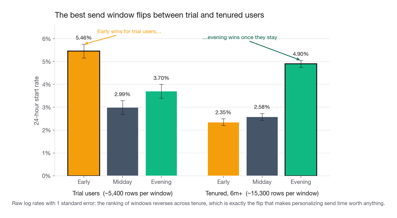
The flips are visible in the raw log with no model at all, which is the cleanest way to defend them under pushback.
| Tenure band | Early | Midday | Evening | Rows per window |
|---|---|---|---|---|
| trial | 5.46% | 2.99% | 3.70% | about 5,400 |
| over_6m | 2.35% | 2.58% | 4.90% | about 15,300 |
Standard errors are roughly 0.3 points on the trial rows and 0.15 on the tenured rows, so both orderings sit far outside noise. Trial users want an early send, tenured users an evening one, and the global average hides it completely. A measured flip like this is the most persuasive artifact you can hand a skeptical PM.
Turning the policy into a number a PM will fund
You now have a predicted 5.78 percent against 4.65 for the best global rule. Do not carry either number into a planning meeting. Neither is measured the way you would want: both are model projections, projections have two failure modes that push upward, and the two rules are not equally exposed to them. Knowing which is which separates a candidate who has shipped this from one who has read about it.
First, an argmax over noisy scores is biased upward. For each cell you took the maximum of 12 estimates, each carrying error, and whichever treatment got the luckiest error is the one you selected. That is the same winner's curse that inflates whichever variant wins a multi-arm test. The bias grows with the number of treatments and shrinks with data per cell, which is why thin cells are dangerous: they do not merely make the policy noisy, they make its projected value overstated.
Second, a well calibrated model is calibrated on the distribution it trained on, and the policy deliberately shifts that distribution by sending far more evening one-line nudges than the rotation did.
The exposure is very uneven, which is the part candidates skip. The policy takes 48 separate maxima over 12 noisy cell estimates, some from cells with a handful of events. The global rule takes one maximum over 12 averages each pooled across all 90,000 rows, so its selection bias is small enough to ignore. That is a reason to replay both the same way, not a prediction of which direction either moves.
The fix for both is to stop projecting and start replaying. Because the rotation was uniform random over the twelve treatments, the holdout contains an unbiased sample of every treatment. Take the rows where the treatment actually received matches what the policy would have chosen, and average the outcome over exactly those rows. That average is an unbiased estimate of what the policy earns.
key = policy[USER + ACT].rename(columns={a: a + "_pol" for a in ACT})
h = hold.merge(key, on=USER, how="left")
match = h[(h["window"] == h["window_pol"]) &
          (h["copy_len"] == h["copy_len_pol"]) &
          (h["hook"] == h["hook_pol"])]

rate = match["started"].mean()
se = np.sqrt(rate * (1 - rate) / len(match))
print(len(match), round(rate, 4), round(rate - 1.96 * se, 4), round(rate + 1.96 * se, 4))
2177 0.0537 0.0443 0.0632Only 2,177 of 27,000 holdout rows match, because a uniform rotation agrees with your policy about one time in twelve. That is the price of an honest offline estimate, and why you hold out generously here. The estimate: 5.37 percent, interval 4.43 to 6.32.
Now put all four numbers side by side.
| Rule | Estimate | How it was obtained | Rows behind it |
|---|---|---|---|
| Today's default (midday, three_line, narrator) | 2.55% | Direct holdout mean | 2,234 |
| Best single global treatment (evening, one_line, plot) | 5.17% | Direct holdout mean | 2,264 |
| Personalized policy, model projection | 5.78% | Weighted mean of predicted argmax | 576 grid rows |
| Personalized policy, replayed | 5.37% | Holdout rows matching the policy | 2,177 |
The projection sits 0.41 points above the replay. Do not present that as the winner's curse measured. It is 0.84 of the replay's own 0.48-point standard error, and the same model under-projects the best global rule, where no selection happened at all, by 0.52 points: 4.65 against a replayed 5.17. A holdout this thin cannot separate selection bias from ordinary calibration error. The sign of the curse you argue from theory; these 2,177 rows do not establish it, and claiming they do invites the fatal follow-up, your own interval is 4.43 to 6.32, so how do you know 0.41 is not noise.
What the replay does settle is which quantity to check. Apply to the bias the rule you apply to lift and compute it on the increment, not the level. The projection said personalization was worth 1.13 points on top of the fixed rule; the replay recovers 0.20, with a standard error near 0.50 once you account for the 1,193 holdout rows the two estimates share, so the interval runs from about minus 0.8 to plus 1.2. That is the number that would have gone in the pitch, and the replay does not confirm it. Say the discipline, not the digits.
The punchline: moving from today's default to the best single treatment is worth 2.62 percentage points, more than doubling the start rate. Moving from that treatment to the full personalized policy is worth 0.20 points, and the two intervals overlap heavily. Ninety-three percent of the available win, on this product with these levers, is a level 0 fix.
Interview tip: Report personalization lift as a delta over the best fixed rule, never over the current rule. Comparing your policy against a stale default is the single most common way personalization results get inflated.
How long each jump takes to prove
Use the two-proportion shortcut: about 16 times p times (1 minus p) divided by the squared difference, per arm.
For the level 0 fix, the pooled rate is about 3.9 percent and the difference 2.62 points, giving roughly 870 users per arm. At 15,000 nudges a week that is powered inside one week.
For the personalization increment, the pooled rate is about 5.3 percent and the difference 0.20 points, giving roughly 200,000 per arm. That is 400,000 nudges, about 27 weeks of full traffic, to detect an effect you already suspect is at the edge of real.
Now run the same formula on the question the taxonomy left open, whether a per-user policy beats this segment table. The rule of thumb puts level 2 at 10 to 30 percent of the total win, here 0.02 to 0.06 points on top of the 0.20. That needs 2.2 million to 20 million per arm, which at 15,000 nudges a week is 6 to 51 years. Offline is no better: a second policy replays through the same matched-row machinery, and this replay's interval already runs 0.95 points either side of the estimate, five times the whole gain in question. At Foxglove's traffic the level 1 against level 2 question is not merely unmeasured, it is unanswerable, and proposing level 2 without that arithmetic is proposing a project nobody can falsify.
One week against half a year is the whole recommendation. Ship the global change now, and either park personalization or restructure it around a cheaper version of the same flip. One is available: fix the copy at one line and personalize only the hook by listening band and the window by tenure. Optimize that restricted family exhaustively and it is worth 5.72 percent against the full policy's 5.78, so dropping copy-length personalization costs 0.06 of the 1.13-point projected increment and takes the creative from twelve pieces to six.
Note the reason, because it is not the obvious one. It is not that copy never flips: it does, on more traffic than either lever you kept. It is that the flip is worth six hundredths of a point and cannot be confirmed from the raw log at 90,000 rows. Among dormant users the observed three-line minus one-line gap is 0.08 points against a standard error of 0.16, where the trial window flip sat several standard errors clear of noise. That is the metric tree's last bullet in the wild, a real difference too thin to act on.
Response modeling versus uplift modeling
Everything above optimized a response rate. That is correct when the treatment is free, which a push notification essentially is: you were sending one anyway, you only chose which. The moment treating a user costs money, response modeling starts recommending the wrong people, and the interviewer will check whether you notice.
The second Foxglove decision: a subscriber opens the cancellation flow, do we offer a free month? The month costs about 12 USD of margin, and only when they stay. A retained subscriber is worth about 88 USD over the next year. The offer was randomized 50/50 across 24,000 cancellation sessions.
rng2 = np.random.default_rng(4471)
M = 24_000
c_ten = rng2.choice(["trial", "under_6m", "over_6m"], M, p=[0.22, 0.34, 0.44])
c_lis = rng2.choice(["none", "light", "steady", "heavy"], M, p=[0.30, 0.32, 0.25, 0.13])
offer = rng2.integers(0, 2, M)
base = (-1.05 + lk({"none": -0.90, "light": -0.20, "steady": 0.50, "heavy": 1.20}, c_lis)
        + lk({"trial": -0.60, "under_6m": 0.0, "over_6m": 0.35}, c_ten))
tau = (lk({"none": 0.05, "light": 0.35, "steady": 0.80, "heavy": 0.10}, c_lis)
       + np.where(c_ten == "trial", -0.60, 0.0))
z2 = base + offer * tau
saves = pd.DataFrame({"tenure": c_ten, "listens": c_lis, "offer": offer,
                      "renewed": (rng2.random(M) < 1 / (1 + np.exp(-z2))).astype(int)})
print(round(saves["renewed"].mean(), 4))0.3018The average effect of the offer is plus 6.16 percentage points on renewal. A naive read says it works, roll it out. Look one level down.
g = (saves.groupby(["tenure", "listens", "offer"], observed=True)["renewed"]
     .agg(["size", "mean"]).unstack("offer"))
g.columns = ["n_ctl", "n_trt", "r_ctl", "r_trt"]
g["uplift_pp"] = 100 * (g["r_trt"] - g["r_ctl"])
g["breakeven_pp"] = 100 * g["r_trt"] * 12.0 / 88.0
g["net_usd"] = (g["uplift_pp"] / 100) * 88.0 - g["r_trt"] * 12.0
print(g[["uplift_pp", "breakeven_pp", "net_usd"]].round(2))| Tenure | Listening band | Users | Uplift (points) | Breakeven uplift | Net per user |
|---|---|---|---|---|---|
| under_6m | steady | 2,031 | +18.53 | 7.23 | 9.95 USD |
| over_6m | steady | 2,664 | +17.50 | 8.67 | 7.77 USD |
| over_6m | light | 3,362 | +11.36 | 5.27 | 5.35 USD |
| under_6m | light | 2,647 | +8.86 | 4.04 | 4.24 USD |
| trial | steady | 1,309 | +3.81 | 3.36 | 0.40 USD |
| over_6m | none | 3,214 | +1.62 | 2.44 | -0.72 USD |
| under_6m | none | 2,429 | +0.55 | 1.78 | -1.08 USD |
| trial | none | 1,605 | -2.73 | 0.62 | -2.94 USD |
| under_6m | heavy | 1,044 | +2.77 | 7.65 | -4.29 USD |
| over_6m | heavy | 1,323 | +3.16 | 8.76 | -4.93 USD |
| trial | light | 1,698 | -4.96 | 1.32 | -5.52 USD |
| trial | heavy | 674 | -9.89 | 4.61 | -12.77 USD |
Print all twelve even when eight tell the story: the rows you drop are the ones a reader needs to reconcile your headline numbers, and one of them is the marginal cell in the policy below.
Three failure modes of response modeling show up in that table.
Sure things. Tenured heavy listeners renew at 61 percent unprompted. The offer moves them 3.2 points, well under the 8.8 it must clear to pay for itself at their acceptance rate. A response model predicts renewal, not the change in renewal, so it ranks this group top and burns money on people who were staying anyway.
Lost causes. Dormant users renew at 16 percent and the offer moves them 1.6 points, inside noise. Cheap to treat, but nothing to buy.
Sleeping dogs. Trial users respond worse to the offer at every listening band except one: minus 2.7 points for dormant, minus 5.0 for light, and almost minus 10 for trial heavy listeners, because the discount reads as a reminder that the trial is about to start charging. The exception is trial steady listeners at plus 3.8 points, barely clear of their 3.4-point breakeven, and the marginal cell in the policy below. This category exists only in an uplift framing: negative effects are invisible when you model the outcome instead of the difference.
| Quadrant | Renews without treatment | Renews with treatment | What the response model does | What you should do |
|---|---|---|---|---|
| Persuadable | No | Yes | Ranks mid, because absolute renewal is unremarkable | Target, this is where all the value is |
| Sure thing | Yes | Yes | Ranks highest, because renewal is highest | Skip, you pay for a decision already made |
| Lost cause | No | No | Ranks lowest | Skip, correctly, but for the wrong reason |
| Sleeping dog | Yes | No | Invisible | Actively exclude, treating them destroys value |
Economics on the whole population: treating everybody nets about 32,000 USD across 24,000 sessions, 1.33 USD per user. Treating only the five positive-net cells covers 50.1 percent of sessions and nets about 70,700 USD, 5.88 USD per targeted user. Half the volume, more than double the money.
Now do to that number what you did to the nudge policy, because it has the same problem. The same twelve estimates chose the cells and priced them, so 70,700 is an in-sample optimum, biased upward the way anything selected on noise is. The offer was randomized, so the honest check is cheap: pick the positive-net cells on one half of the sessions, score them on the other, and repeat enough times that the answer is not one lucky split.
def cell_net(df):
    t = (df.groupby(["tenure", "listens", "offer"], observed=True)["renewed"]
         .agg(["size", "mean"]).unstack("offer"))
    t.columns = ["n_ctl", "n_trt", "r_ctl", "r_trt"]
    t["net"] = (t["r_trt"] - t["r_ctl"]) * 88.0 - t["r_trt"] * 12.0
    t["users"] = t["n_ctl"] + t["n_trt"]
    return t

rs = np.random.default_rng(99)
ins, out = [], []
for _ in range(200):
    fold = rs.integers(0, 2, len(saves))
    pick, score = cell_net(saves[fold == 0]), cell_net(saves[fold == 1])
    chosen = pick.index[pick["net"] > 0]
    if len(chosen) == 0:
        continue
    ins.append(np.average(pick.loc[chosen, "net"], weights=pick.loc[chosen, "users"]))
    out.append(np.average(score.loc[chosen, "net"], weights=score.loc[chosen, "users"]))
print(round(np.mean(ins), 2), round(np.mean(out), 2),
      round(100 * (1 - np.mean(out) / np.mean(ins)), 1))
5.74 5.17 10.0The in-sample figure averages 5.74 USD per targeted user, the honest one 5.17, a 10 percent overstatement. Each selection there runs on 12,000 sessions rather than 24,000, so it is noisier than the real procedure and 10 percent is the pessimistic end. Either way it is the same order as the gap on the nudge policy, so quote it the same way.
What keeps the conclusion standing is concentration, not precision. The marginal cell is trial steady listeners at plus 0.40 USD per user against a standard error near 2.00, a coin flip, and the four above it carry 99 percent of the money. Drop it and the total moves 70,700 to 70,100 while coverage falls from 50.1 percent to 44.6, so it threatens the "half the volume" framing and not the "double the money" punchline. Name it before a PM finds it.
Interview tip: The instant a treatment has a unit cost, say the words "I would model uplift, not response" and name sleeping dogs. Interviewers listen for whether you know a positive-response segment can still be a negative-value segment.
How to actually estimate uplift
That table is the segment-level estimator, and for a handful of cells with thousands of users each it is often all you need. When cells get thin, three model-based options:
Two models (T-learner): fit one model per arm and difference the predictions. Simple, and it doubles your variance because you are differencing two noisy surfaces.
One model with a treatment interaction (S-learner): include the treatment flag as a feature and predict twice, on and off. Lower variance, but a tree learner may never split on the flag when main effects dwarf the interaction, and your uplift estimates come back identically zero.
Transformed outcome: with 50/50 randomization, label treated rows plus 2 times the outcome and control rows minus 2 times the outcome, then fit an ordinary regression. Its conditional mean is the uplift, so any regressor works. Noisy per row, unbiased in aggregate, easy to explain out loud.
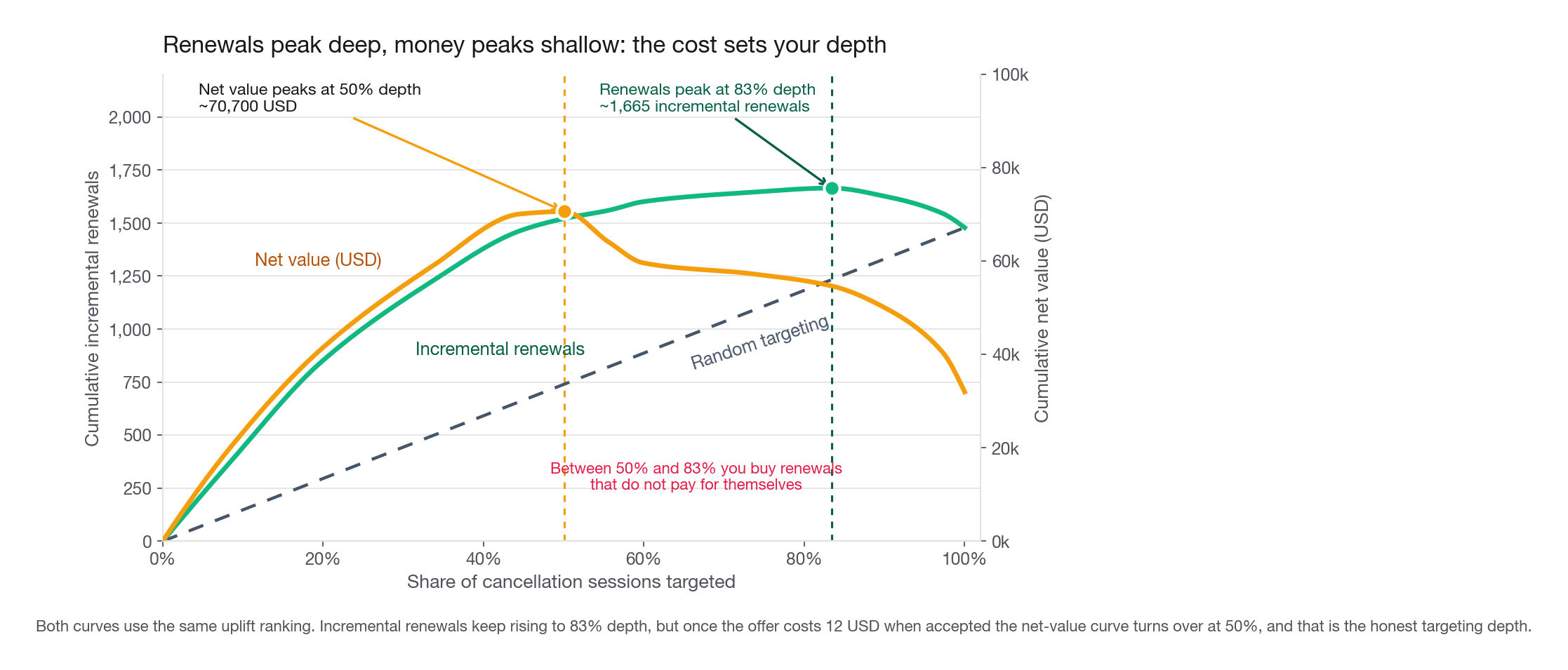
Evaluate with a cumulative-uplift curve, not AUC. Sort by predicted uplift and at each depth take the observed treated rate minus the control rate among users covered so far, times the number covered. A useful model rises fast, then flattens or turns down once it starts adding cells with no effect or a negative one.
Read the depth off the right curve, though, because this is the section's own point. Ranked by uplift, incremental renewals here climb to about 1,665 at 83 percent of sessions and only turn down once the trial cells enter, against 1,478 for random targeting at full coverage. But renewals are not the objective when the offer costs money. Plot the same ranking against net value, uplift times 88 USD minus the treated acceptance rate times 12, and it peaks far earlier, at 50.1 percent and about 70,700 USD, exactly the positive-net policy above. The gap between 83 and 50 percent is the breakeven uplift made visible: every session in it buys a renewal that does not pay for itself. When the treatment has a unit cost, the second curve sets your depth and the first flatters it.
When personalization is not worth the complexity
Saying no is a scored answer. Here is the checklist that produces a defensible one.
Three situations where the answer is no.
The levers do not interact with the user. If every cell picks the same treatment, personalization is a rebranded config change. Measure the flip rate and you know within an afternoon.
The treatment data is not randomized. If the old rule already varied by user, the differences you find describe that rule, not user preference. Run a rotation, which is what Foxglove's six weeks were for, or treat your policy as a hypothesis to test rather than a lift to project.
The ceiling is too low to matter. Dormant users top out around 4 percent even on their best nudge, against 14 percent for the average heavy listener. Tripling off a low base is still a low base, so change the instrument rather than the message.
Common traps
Comparing the policy to today's default instead of the best fixed rule. This inflates reported lift by whatever the stale default was costing. Always report two deltas.
Projecting the model's predicted rate as the business impact. The argmax of noisy scores is biased upward, and a calibrated model is calibrated only on the distribution it saw. Replay on held-out rows where the logged treatment matches the policy choice, and quote that.
Enumerating observed combinations instead of the full grid. De-duplicating the training frame gives you what was sent, not what is available. Build the cross product explicitly and score all of it.
Averaging cell predictions without population weights. Averaging 48 cells equally lets a cell with 0.7 percent of traffic count as much as one with 7.5 percent, quietly turning your headline into fiction.
Personalizing on an attribute that changes levels but not rankings. Market moved Foxglove's response rate by about 1.3 points across markets and interacts with no lever, yet the fitted policy still picked a different treatment across markets in 7 of 12 user groups. Such attributes belong in the model as features, not in the personalization key, and the flips they seem to produce are a signal that your flip rate is noise-inflated.
Using a response model when treating a user costs money. It targets sure things, misses persuadables, and cannot see sleeping dogs. Switch to uplift, and evaluate with a cumulative-uplift curve rather than AUC.
Treating a policy as permanently correct. Preferences drift with the product, the season, and the audience mix, and a policy never refit becomes a stale global rule with extra steps. Put a refresh cadence and a holdback arm in the design from day one.
Quick self-check
Answer these out loud, in full sentences, as you would to an interviewer.
A colleague reports that personalizing send time raised the start rate from 2.6 to 5.4 percent. What single question do you ask before believing personalization caused it, and what do you expect the answer to reveal?
Your model separates high from low responders with an AUC of 0.82. Why does that number tell you nothing about whether personalization pays, and which statistic does?
You have 60,000 events at a 2 percent response rate, 5 user attributes with 3 levels each, and 8 treatments. How many cell-and-treatment combinations, roughly how many responses each, and what does that force you to change?
The historical policy was not randomized: growth already sent tenured users in the evening. What breaks in the argmax approach, and what do you do instead?
A retention offer shows a plus 4 point average effect. One segment renews at 70 percent without it and 74 percent with it. The offer costs 12 USD when accepted and a retained subscriber is worth 88 USD. Target that segment or not, and show the arithmetic.
Offline replay says the policy is worth 5.4 percent against 5.2 for the best fixed rule. How many users per arm does the confirming test need, how long is that at your traffic, and what do you tell the PM?