4.4 Novelty Effects, Guardrails, and Ship Rules
Find the core decision, design, or behavior signal.
Turn the lesson into a concise response blueprint.
Name the trap you would avoid in a real interview.
Use these checkpoints as your reading path before diving into the full lesson.
- 1Why this matters in interviews
- 2Two things happen when users meet somet...
- 3Curiosity inflation
- 4Reluctance to relearn
- 5The honest framing: you ran two treatments
A test comes back green: primary metric up 2.8 percent, p-value 0.0045, product manager already drafting the launch post. Your job in the next ten minutes is to decide whether that number will still be there in six weeks, and whether anything else moved in a direction that should stop the launch anyway. This lesson gives you both halves, plus the artifact that makes the decision boring: a ship rule written before a single user was assigned.
Why this matters in interviews
Everything so far in this section produced a number: pick the decision, size the test, randomize cleanly, run the comparison. This lesson is about not being fooled by that number. Interviewers probe it in three shapes.
The first is the trap prompt. "Engagement is up 4 percent after two weeks. Do you ship?" The candidate who says yes has failed. So has the candidate who says "no, always run longer," because that answer carries no cost model. The wanted answer names the specific alternative explanation, gives a test that separates it from the real one, and prices the extra runtime.
The second is the guardrail prompt. "Your primary metric is up and your support contact rate is up 12 percent. What now?" This tests whether you understand that a guardrail is not a second success metric. It has a different null hypothesis, a different threshold, and a different consequence.
The third is the process prompt. "How do you stop people cherry-picking results?" The answer is not a statistical technique. It is a document, written before the test starts.
Interview tip: When you hear a lift quoted alongside a run length shorter than about three weeks, your first sentence should be "how does that lift look by days since a user first saw the feature?" That single question signals more experimentation maturity than any amount of vocabulary.
The recurring failure across all three is treating a result as a fact rather than an estimate of a quantity you had to define. The rest of this lesson is that definition work.
Two things happen when users meet something new
Curiosity inflation
Ship a visibly new control on a screen people already use daily and some fraction will tap it because it is unfamiliar, not because it is useful. That tap is real behavior, it lands in your logs, and at the row level it is indistinguishable from one that reflects genuine value.
The trouble is that this curiosity budget is finite and non-renewing. Each user spends it once. If your measurement window overlaps the period when a large share of your treatment group is spending theirs, the average you compute blends the durable effect with a one-time exploration burst. You are trying to buy the steady state, because that is what everyone will be living in a month after launch.
This is worst where the headline metric counts interactions: sessions, taps, pages, plays, messages. It is milder on metrics with a natural per-user ceiling, milder still on metrics gated by money.
Reluctance to relearn
The mirror image exists too. Move a button people have used four hundred times and they slow down for a while, not because the new spot is worse but because muscle memory points at the old one. Measured during that adjustment, a good change reads as a loss.
This bites less often than curiosity inflation for a structural reason: it needs a change big enough to disrupt a learned habit, and changes that big are usually redesigns with their own rollout plan rather than a two-week test. But on a navigation overhaul or an editor rewrite, expect it, and expect it strongest in your heaviest users.
| Property | Curiosity inflation | Reluctance to relearn |
|---|---|---|
| Direction of the bias | Treatment looks better than it is | Treatment looks worse than it is |
| Who feels it | Users who already had a habit | Users who already had a habit |
| Typical triggers | New surface, new badge, new recommendation shelf | Moved controls, renamed concepts, redesigned flows |
| Metric families most affected | Interaction counts, time on surface | Task completion time, error rate, first-week retention |
| Rough decay window | 3 to 10 days of exposure | 2 to 6 weeks of exposure |
| What it does to your decision | Ships a change that later evaporates | Kills a change that would have won |
The honest framing: you ran two treatments
Both are instances of a general problem, and saying it this way in an interview is worth a lot. Your treatment arm did not receive one intervention. It received two: the feature, and the experience of meeting something unfamiliar. Control received neither. A difference of means cannot unbundle two treatments, so you separate them by design.
The same logic reaches well beyond interface changes. Offer one arm a 20 percent discount and you have bundled "this is cheaper" with "I was singled out for a deal." Whenever you can name a second thing that arrived alongside your feature, you have a novelty-shaped problem even if nobody calls it that.
Interview tip: Say the phrase "the treatment arm got two changes, not one" out loud. It reframes novelty from a piece of trivia into a design flaw you know how to attack.
The running example
Tessera is a mobile board-game platform. Players browse a lobby, pick an opponent, and play asynchronous matches. The team has built Quick Match, one button that instantly pairs you with a similarly ranked opponent instead of making you scroll. It is a new, visible control on the home screen of every existing player.
The experiment runs 21 days. Assignment is at the player level, and a player enters the analysis the first day they open the app after launch, which is the first day they could have seen the button. The primary metric is matches started per player per day, averaged within a player and then across players. The trust team's guardrail is the rate at which players report an opponent, since faster pairing may put people in front of opponents they would have avoided.
This block builds a deterministic player-day panel with that schema. Every later block assumes panel exists.
import numpy as np
import pandas as pd

SEED = 20260826
rng = np.random.default_rng(SEED)

N_PLAYERS, DAYS = 12_000, 21
tenure = np.where(rng.random(N_PLAYERS) < 0.22, "new", "returning")
variant = rng.integers(0, 2, N_PLAYERS)
first_day = np.where(tenure == "new", rng.integers(1, DAYS + 1, N_PLAYERS),
                     np.minimum(rng.geometric(0.55, N_PLAYERS), 6))
skill = rng.lognormal(0.0, 0.45, N_PLAYERS)

n_days = DAYS + 1 - first_day
pid = np.repeat(np.arange(N_PLAYERS), n_days)
exposure_day = np.concatenate([np.arange(k) for k in n_days])
panel = pd.DataFrame({
    "player_id": pid, "variant": variant[pid], "tenure": tenure[pid],
    "first_day": first_day[pid], "exposure_day": exposure_day,
    "calendar_day": first_day[pid] + exposure_day,
})

base = np.where(panel["tenure"] == "returning", 1.35, 0.95) * skill[pid]
weekend = 1.0 + 0.18 * (panel["calendar_day"] % 7).isin([5, 6])
novelty = np.where(panel["tenure"] == "returning",
                   0.095 * np.exp(-panel["exposure_day"] / 4.0), 0.0)
rate = base * weekend * (1.0 + panel["variant"] * (0.015 + novelty))

panel["matches_started"] = rng.poisson(rate)
panel["minutes_played"] = np.round(panel["matches_started"] * rng.gamma(6.0, 1.4, len(panel)), 1)
panel["reported"] = (rng.random(len(panel)) < 0.004 + 0.0016 * panel["variant"]).astype(int)
print(panel.shape)
(218033, 9)Columns: player_id, variant (1 for Quick Match), tenure (did the account exist before the test), first_day, exposure_day (days since first exposure, from 0), calendar_day, matches_started, minutes_played, reported.
The generator hides a durable 1.5 percent lift plus a curiosity burst that halves every few days, so we can grade each method by where it lands.
The naive read
Roll the panel up to one row per player and compare.
from scipy import stats

player = (panel.groupby(["player_id", "variant", "tenure"], as_index=False)
                .agg(days=("exposure_day", "size"),
                     matches=("matches_started", "sum"),
                     reports=("reported", "sum")))
player["mpd"] = player["matches"] / player["days"]

def compare(df, col="mpd"):
    t = df.loc[df.variant == 1, col]
    c = df.loc[df.variant == 0, col]
    se = np.sqrt(t.var(ddof=1) / len(t) + c.var(ddof=1) / len(c))
    d = t.mean() - c.mean()
    return pd.Series({"n": len(t) + len(c), "control": c.mean(),
                      "lift_pct": 100 * d / c.mean(),
                      "ci_lo": 100 * (d - 1.96 * se) / c.mean(),
                      "ci_hi": 100 * (d + 1.96 * se) / c.mean(),
                      "p": stats.ttest_ind(t, c, equal_var=False).pvalue})

print(compare(player).round(4).to_string())
n 12000.0000
control 1.4704
lift_pct 2.8297
ci_lo 0.8794
ci_hi 4.7800
p 0.0045Matches started per player per day rose 2.83 percent, interval roughly 0.9 to 4.8 percent. Nothing here is wrong: randomization is clean, the unit of analysis matches the unit of assignment, the interval is honest about its own width. It is also 89 percent too big, and you cannot tell that from this output.
A weak answer stops here and hedges: "of course we should watch out for novelty effects." That sentence costs nothing and buys nothing. The stronger answer produces the diagnostic.
Diagnostic one: split on who could feel the novelty
Curiosity inflation needs a baseline to deviate from. A player who joined Tessera yesterday has no memory of a lobby without a Quick Match button; the feature is not novel to them, it is simply how the product works. A real effect should appear for brand new accounts too. Curiosity concentrates in accounts that predate the change.
rows = []
for name, grp in player.groupby("tenure"):
    r = compare(grp)
    r.name = name
    rows.append(r)
print(pd.DataFrame(rows).round(4).to_string())
n control lift_pct ci_lo ci_hi p
new 2614.0 1.1123 2.1209 -2.6735 6.9152 0.3860
returning 9386.0 1.5688 3.1584 1.0974 5.2194 0.0027Returning players are up 3.16 percent with p equal to 0.0027, inside a Bonferroni-corrected threshold of 0.025 for two pre-registered splits. New players are up 2.12 percent with p equal to 0.386, clearing nothing. This is where most candidates declare victory and where a good interviewer pounces.
The trap inside the diagnostic
"Not significant for new players" is not the same claim as "no effect for new players." Look at the interval: minus 2.7 percent to plus 6.9 percent. That arm has 2,614 players. The smallest lift it could reliably detect is around 6.9 percent relative. The true durable effect in this simulation is 1.5 percent. The new-player split was never capable of seeing it, so its silence is uninformative.
The correct reading is narrower: the data fit a curiosity story and equally fit a small real effect this split cannot resolve. Both stay live, and you need a diagnostic that does not discard 78 percent of your sample.
Interview tip: Whenever you report a null on a subgroup, report its detectable effect size in the same breath. "Flat for new users, but that slice could only have caught something above 7 percent" is the sentence that separates a senior candidate from a confident one.
Run this split even when novelty is not a concern. A change that only helps people who already love your product is how a team tunes itself into a local optimum, and the new-account arm is a cheap standing check against that.
Diagnostic two: the decay curve
The stronger tool measures time in days since that player first saw the feature rather than in calendar days. Call it the exposure day: the same alignment you use for retention cohorts, applied to an experiment.
Calendar day and exposure day are not the same axis. Players enter on different dates, so on calendar day 12 your treatment arm holds people on their first day of exposure and people on their twelfth. Slicing by calendar day averages those, and the mix drifts as the test runs, so the trend confounds the decay you want with a composition shift you do not.
ret = panel[panel["tenure"] == "returning"].copy()
ret["week"] = ret["exposure_day"] // 7
wk = ret.groupby(["week", "variant"])["matches_started"].mean().unstack()
wk.columns = ["control", "treatment"]
wk["lift_pct"] = 100 * (wk["treatment"] / wk["control"] - 1)
print(wk.round(3).to_string())
control treatment lift_pct
week
0 1.563 1.656 5.946
1 1.572 1.602 1.926
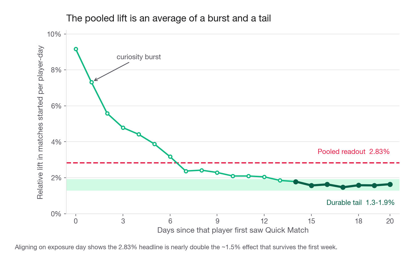
2 1.570 1.590 1.296In a player's first week with the button they start 5.9 percent more matches, in the second 1.9 percent, in the third 1.3 percent. The control column barely moves, which is what you want: the decay belongs to the treatment, not to a seasonal artifact hitting both arms.
Now you can be precise. The pooled 2.83 percent is an average of a large opening burst and a small persistent tail, weighted by how much of the window sat in each regime. The number to carry into a forecast is the tail, near 1.3 to 1.9 percent.
Reading the shape
Three shapes come up, each implying a different action.
A curve that starts high and settles onto a positive plateau is the ordinary case, real effect plus curiosity, so take the plateau. A curve that starts high and decays to zero is a pure exploration burst, and there is nothing to ship; say so plainly rather than proposing to run longer, because more data only estimates zero more precisely. A curve that starts negative and climbs is reluctance to relearn, and there running longer genuinely is the right call.
Name the limit out loud: you cannot separate these with under about two weeks of exposure per user, and a curve read off three days is noise with a slope.
Choosing a run length once you know novelty is in play
The obvious fix, run everything for six weeks, is unaffordable. A team shipping 40 experiments a quarter through one traffic pool cannot triple every duration and still decide anything. The question is which tests earn the extra time. Power and duration mechanics belong to the sizing lesson; what changes here is that a chunk of your data is deliberately unusable for the headline estimate.
The burn-in window
The standard move is a pre-registered burn-in: declare before launch that each user's first N exposure days are excluded from the primary analysis. It is per user, not per calendar date, so a player arriving on day 9 still has their own first seven days trimmed.
warm = panel[panel["exposure_day"] >= 7]
warm_player = (warm.groupby(["player_id", "variant", "tenure"], as_index=False)
                   .agg(days=("exposure_day", "size"),
                        matches=("matches_started", "sum")))
warm_player["mpd"] = warm_player["matches"] / warm_player["days"]
print(compare(warm_player).round(4).to_string())
n 11126.0000
control 1.4987
lift_pct 1.5925
ci_lo -0.4633
ci_hi 3.6482
p 0.1290The point estimate drops to 1.59 percent. Resist reading that as a bullseye. A burn-in shrinks novelty bias, it does not zero it, because an exponential decay never actually lands. The burst here decays as exp(minus exposure_day over 4), so on exposure day 7, the first day this analysis keeps, 1.65 percentage points of curiosity are still in the treatment arm, more than the 1.5 point durable effect itself. Averaged over the days that survive the trim, this comparison targets about 2.0 percent, not 1.5. The decay curve above says so visually: at day 7 the line has not yet come down into the shaded tail band.
What the trim bought is about three quarters of the bias: the untrimmed comparison targets 3.25 percent, the trimmed one 1.98, against a durable truth of 1.5. Our 1.59 is one draw from an interval over four points wide and it landed low. Re-run the block on twenty other seeds and the trimmed estimate averages 2.12 percent, clearing p equals 0.05 nine times. Read residual bias off the design, never off the point estimate you happened to draw.
The inconclusiveness is still the most instructive part, but it is a sample-size fact, not evidence the estimate is right: p equals 0.129, interval crossing zero. The trim took a third of the observations with the bias, and the remainder was sized against a 2.8 percent signal, not a 1.6 percent one.
Pick the window against the decay constant, not by eye. Fit the curve to a plus b times exp(minus d over tau), set the burn-in near three to four times tau, and write down the residual you accept. "The first day it looks flat" fires days too early, because per-day noise swamps the slope: exposure day 10 reads minus 0.15 percent and day 14 reads plus 4.7 percent against true values of 2.28 and 1.79. When the calendar cannot afford three to four times tau, fit the decay and report the asymptote instead of trimming to it.
The lesson is sequencing. If you expect novelty, the burn-in belongs in the sizing calculation, not in the post-hoc analysis. Powering for 1.6 percent on post-burn-in data alone needs roughly four times the players that 3 percent needs, plus the calendar time for every user to clear their own window.
Interview tip: If you propose a burn-in window, immediately state the sample-size consequence: "the first week is excluded, so I size the test on the remaining exposure days and the run gets about 60 percent longer."
| Approach | What you gain | What it costs | Reach for it when |
|---|---|---|---|
| Run the standard window, report pooled | Speed, simplicity | Biased high on any visible new surface | The change is invisible to users, such as a ranking backend swap |
| Pre-registered burn-in, size for the tail | Most of the bias removed, the residual set by how the burn-in compares to the decay constant | Roughly 1.5x to 2x the sample and calendar time | The change is visible and the decision is expensive to reverse |
| Read the exposure-day curve, ship on the tail | Cheap, uses all the data, shows the shape | The tail estimate is the noisiest part of the curve | You need a fast directional read and can follow up |
| New-accounts-only readout | Structurally free of curiosity inflation | Small arm, and new users may respond differently anyway | New-account volume is large relative to the base |
| Long-term holdback after launch | Measures the true steady state at full scale | Slow, needs holdback infrastructure | The feature is strategic and you must know its real value |
The holdback is the answer interviewers most like to hear and the one candidates least often give. Ship to 95 percent, keep 5 percent on the old experience for eight weeks, read the difference at week eight. It answers the question the experiment could not, it does not delay the launch, and it costs a slice of upside instead of a slice of time. Its own hazards get a full treatment in the long-term metrics lesson later on.
Peeking, and what it does to your error rate
A dashboard that recomputes the p-value nightly is an efficient machine for manufacturing false positives, because the 0.05 threshold assumes exactly one look at a sample size fixed in advance.
The intuition: a running difference wanders, so 14 nightly looks give it 14 chances to poke outside the boundary. Stopping the moment it does is a rule with a far higher error rate than the one you think you are running. Simulate it.
rng2 = np.random.default_rng(4242)
SIMS, LOOKS = 20_000, 14
inc = rng2.normal(0.0, 1.0, (SIMS, LOOKS))
z = np.cumsum(inc, axis=1) / np.sqrt(np.arange(1, LOOKS + 1))
crossed = np.abs(z) > 1.96

print("stop at any nightly look:", round(crossed.any(axis=1).mean(), 3))
print("look only at the end    :", round(crossed[:, -1].mean(), 3))
for k in (2, 3, 7):                      # equally spaced in information
    idx = np.rint(np.arange(1, k + 1) * LOOKS / k).astype(int) - 1
    print(f"  {k} looks:", round(crossed[:, idx].any(axis=1).mean(), 3))
for c in (2.55, 2.60, 2.65, 2.70):
    print(f"  boundary {c}:", round((np.abs(z) > c).any(axis=1).mean(), 3))
stop at any nightly look: 0.221
look only at the end : 0.05
2 looks: 0.083
3 looks: 0.105
7 looks: 0.167
boundary 2.55: 0.062
boundary 2.6: 0.055
boundary 2.65: 0.048
boundary 2.7: 0.043Under a true null, one look at the end is wrong 5 percent of the time, as designed. Nightly looks with a stop-on-significance rule are wrong 22 percent of the time, and even two looks raise it by about two thirds.
| Number of looks with a 1.96 boundary | False positive rate under the null |
|---|---|
| 1 (fixed horizon) | 0.050 |
| 2 | 0.083 |
| 3 | 0.105 |
| 7 | 0.167 |
| 14 (nightly for two weeks) | 0.221 |
Those looks are spaced equally in information, the assumption behind every published sequential-testing table: two looks means half the sample and the end, not a peek on night one. Fourteen does not divide by three, so that row uses the closest schedule available, nights 5, 9, and 14, and reads 0.105 rather than the textbook 0.107. Schedule matters: anchor the series on night one instead and two looks reads 0.097, because a look at a fourteenth of the information is nearly independent of the last one.
The last four lines show the repair for a constant boundary: widen it to about 2.65 and the fourteen-look procedure returns to roughly 5 percent. That constant-threshold family is one of the classic group sequential designs, and it makes the price explicit. You keep the option to stop early and pay for it with a wider bar at every look, including the final one.
Three defensible policies
A fourth policy is legitimate and often overlooked: watch guardrails nightly with no early-stopping rule on the primary metric. Nobody objects to a safety monitor. The inflation matters only when a look feeds a stopping decision on the metric you are trying to prove.
Interview tip: If asked "can I stop early because it already looks significant?", answer with the mechanism, not a rule: "under a null, the running estimate crosses the 5 percent boundary about one time in five if you check nightly, so early stopping needs a wider boundary that I would have to plan in advance."
Multiple comparisons inside a single experiment
Peeking is one flavor of a bigger issue. Count the tests a typical readout performs: one primary metric, six guardrails, four segments, fourteen nightly looks. Treat each as an independent decision at 0.05 and you are running over a hundred tests and calling the largest a discovery.
The fix is not to correct everything at 0.05 divided by 100, which makes the test useless. It is to sort the comparisons into families with different jobs.
| Family | Typical size | Error control | Consequence of a hit |
|---|---|---|---|
| Primary metric | 1 | Full alpha at 0.05, one look | Drives the ship decision |
| Pre-registered segments | 2 to 4 | Bonferroni within the family | Drives a scoped ship, or a follow-up test |
| Guardrails | 4 to 8 | One-sided, looser alpha such as 0.10 | Blocks the launch or forces mitigation |
| Exploratory metric wall | 30 to 300 | False discovery rate control, or none | Generates hypotheses only, never conclusions |
Two rows there surprise people.
The guardrail family gets a looser threshold, not a stricter one. The asymmetry is deliberate: a false alarm on a guardrail costs a delayed launch, while a miss costs shipping a harm to everyone. Errors with different prices should not share a threshold.
The exploratory wall is not corrected because it is not making decisions. Slicing 200 metrics by country and finding four that moved is a hypothesis generator, which is fine and useful. It becomes misconduct the moment one of those four appears in a launch memo as evidence. Segments, by contrast, must be listed before launch, because a segment chosen after the fact has an unknown number of silently discarded siblings and its p-value cannot be read.
The pattern generalizes: look at anything, conclude only from what you committed to.
Guardrails
A guardrail is a metric you do not expect to improve and whose degradation you will not accept in exchange for the win. Guardrails invert the hypothesis. For your primary metric you ask "can I rule out that this did nothing?" For a guardrail you ask "can I rule out that this did meaningful harm?" Different questions, different failure modes, and conflating them is the most common error in this area.
What belongs on the list
| Category | Tessera example | Why it can block a launch |
|---|---|---|
| Counter-metric to the primary | Matches abandoned before the first move | Quick pairing could inflate starts while producing worse matches |
| Trust and safety | Player reports per player-day | Faster pairing may expose people to opponents they would have avoided |
| Business north star | Weekly paying-player rate | Engagement that does not convert is not a win |
| Reliability and latency | p95 lobby load time | A slower home screen taxes every user, not just feature users |
| Cost | Matchmaking compute cost per match | An effect bought with a 3x cost increase is not an effect |
| Support load | Contacts per thousand active players | A large jump usually means something is confusing or broken |
Keep the list short, stable across experiments, and owned by someone outside the team running the test. A guardrail the experimenting team can quietly delete is decoration.
Thresholds, not significance
The wrong rule is "block if the guardrail moved significantly." Under it a large test blocks on a 0.2 percent regression nobody cares about, and a small test waves through a 15 percent regression it lacked power to see. Both backwards.
The right rule states a margin: the largest degradation you would tolerate. Tessera's trust team sets 15 percent relative on the report rate. The question becomes whether the data rule out harm bigger than the margin, which is one-sided and about the margin, not about zero.
Stop there and you have swapped one power problem for its mirror image: a guardrail underpowered against its own margin never clears. So the readout has three states, not two, all against the margin M rather than zero.
Upper bound below M: cleared, the data rule out harm you would care about
Lower bound above M: demonstrated breach, the harm exceeds your tolerance
Interval straddling M: uninformative, this test could not answer the question
The third state is the one nobody writes down. Tessera's pre-registered report-rate estimand has a relative standard error of 6.8 points, so its interval reaches 13.3 points either side, and a feature whose true effect is exactly zero clears only 60 percent of the time: two harmless launches in five blocked by a guardrail that measured no harm. An uninformative guardrail still stops a full ramp, since for a safety metric the burden of proof runs toward showing non-inferiority; what changes is the response, and the decision table below carries both branches.
The real repair is at design time: publish the minimum detectable harm next to every margin and require the expected half-width to sit under it. This page's own output shows the cost of skipping that. Mean-of-rates has a half-width of 15.8 points against a 15 percent margin, so pre-registering that definition would have made clearing the guardrail require measuring an improvement. When the check fails, widen the margin, pick a lower-variance estimand, extend the window, or demote the metric to informational.
Fix one inconsistency while you are here: the families table below prescribes a one-sided alpha near 0.10 for guardrails, while compare() hard-codes 1.96 and hands you a 97.5 percent one-sided bound. Pick one and say which. This verdict does not move, but the choice is not cosmetic: at one-sided 0.10 the same margin blocks a harmless feature 18 percent of the time instead of 40, and it flips mean-of-rates from futile to usable, half-width 10.3 against a margin of 15.
The estimand trap
Before running that check, decide what "the report rate" means. It has at least three defensible definitions, each saying something different about the same data.
tot = panel.groupby("variant")["reported"].agg(["sum", "size"])
p1 = tot.loc[1, "sum"] / tot.loc[1, "size"]
p0 = tot.loc[0, "sum"] / tot.loc[0, "size"]
se = np.sqrt(p1 * (1 - p1) / tot.loc[1, "size"] + p0 * (1 - p0) / tot.loc[0, "size"])
print("ratio of totals  %+.1f%%  CI [%.1f, %.1f]"
      % (100 * (p1 / p0 - 1), 100 * (p1 - p0 - 1.96 * se) / p0,
         100 * (p1 - p0 + 1.96 * se) / p0))

player["rate"] = player["reports"] / player["days"]
player["any_report"] = (player["reports"] > 0).astype(int)
cols = ["lift_pct", "ci_lo", "ci_hi", "p"]
print("mean of rates    ", compare(player, "rate")[cols].round(3).to_dict())
print("any report       ", compare(player, "any_report")[cols].round(3).to_dict())

def cluster_se(arm):                     # delta method at the randomization unit
    g = player[player["variant"] == arm]
    y, n = g["reports"].to_numpy(float), g["days"].to_numpy(float)
    resid = y - (y.sum() / n.sum()) * n
    return np.sqrt(len(y) * resid.var(ddof=1)) / n.sum()

print("ratio-of-totals SE  naive %.6f  player-clustered %.6f"
      % (se, np.sqrt(cluster_se(1) ** 2 + cluster_se(0) ** 2)))
ratio of totals +22.7% CI [9.0, 36.4]
mean of rates {'lift_pct': 13.746, 'ci_lo': -2.05, 'ci_hi': 29.542, 'p': 0.088}
any report {'lift_pct': 21.017, 'ci_lo': 7.732, 'ci_hi': 34.303, 'p': 0.002}
ratio-of-totals SE naive 0.000292 player-clustered 0.000291Three numbers: plus 22.7, plus 13.7, plus 21.0 percent. Two clear a 0.05 bar and one does not.
Now grade them against the generator, as we graded everything else here. It hides a 40 percent lift in the per-day report rate, and all three estimands are worth roughly that in truth: 40 percent for the ratio of totals, 40 for the mean of per-player rates, 38 for the binary, which runs lower because a player with more days has more chances to trip it. Every printed interval misses. On an event this rare, one run of 12,000 players cannot resolve the estimand question at all, and the 9-point spread between 13.7 and 22.7 is sampling noise on a thousand reports rather than the weighting doing work. Which sharpens the argument for pre-committing: after the fact nobody, your reviewer included, can separate noise-shopping from estimand-shopping.
The weighting differences are real in production even though this panel is too clean to show them. The ratio of totals weights each player by days in the test, so accounts that entered early carry more weight. The mean of per-player rates weights players equally and inherits the huge variance of a rare event measured on individuals. The binary asks whether a player reported at all, and is most stable precisely because it discards magnitude, which is what makes it robust to one prolific reporter. There is none here to be robust against: the busiest account filed three reports, because reported is drawn independently per row with a probability depending on nothing but the variant. Real report data is not like that.
The same artifact hides a bug, and it is the standard ratio-metric follow-up. That interval uses a binomial standard error over 218,033 player-days while assignment was at the player, so it counts every player-day as an independent trial. A ratio whose numerator and denominator are both random at the randomization unit needs a clustered variance: the delta method on each player's reports-and-days pair, or a bootstrap over players. The block prints both and they agree to within half a percent, precisely because the generator has no player-level report propensity. Give players one, a lognormal multiplier at sigma near 1.6, and the busiest account files closer to a dozen reports than three, the design effect climbs to about 1.8, and the honest interval runs a third wider. So the certification is narrow: all three point estimates are correct and both player-level intervals are specified right, but the ratio-of-totals one is not. Coinciding on synthetic data is why a demo cannot show you this.
An analyst who computes all three after the results land and reports the one matching their prior is not committing fraud, but is choosing the verdict. That is why the ship rule fixes the estimand before launch. For a rare safety event the per-player binary is usually the right pre-commitment: robust, readable as "how many people had a bad time," and hard to distort with one heavy account.
Take the pre-registered version: a 21 percent increase, interval 7.7 to 34 percent, against a 15 percent margin. Be precise about which state that is. The interval straddles 15, so this is not proof of harm beyond tolerance; it is a failure to rule such harm out, with a point estimate already past the margin. For a safety guardrail that is enough to stop the ramp, and the honest sentence names the state rather than borrowing the language of proof.
Interview tip: State a guardrail verdict as a sentence about the margin, not the p-value, and name which of the three states you are in: "the interval straddles our 15 percent tolerance, so we cannot rule out harm past it, and this does not ship in its current form."
What a failed guardrail actually triggers
Not automatically "kill it." Guardrails come in tiers, written next to the metric.
A hard stop tier, usually safety, legal, and severe reliability regressions, halts the experiment automatically when breached, with no meeting. Say in advance which metrics can page an on-call engineer and turn the feature off. A blocking tier, most guardrails, means the launch waits until the regression is fixed or explicitly accepted by a named owner. An informational tier just gets reported; if a metric never blocks anything, call it context, not a guardrail.
Tessera's report-rate guardrail sits in the blocking tier, and since it could not clear its margin the launch waits. The mechanism suggests the mitigations: drop previously blocked opponents from the Quick Match pool, or add a confirmation step before pairing. Both are testable next, and both keep most of the 1.5 percent durable lift.
The ship rule
Everything above collapses into one artifact: a short document agreed before the first assignment that makes the readout mechanical.
The last two lines do the most work and are usually missing.
An experiment has three outcomes, not two: a win, a loss, and a failure to distinguish the win from nothing. If the plan is silent on the third, it becomes an argument, and arguments are won by whoever wants it more. Write the branch: extend by a defined number of days, ship on strategic grounds the metric does not capture, or drop it. Any of those is defensible; deciding afterward is not. Naming a decider prevents the other failure, the readout that circulates for three weeks while everyone reinterprets it.
The decision matrix
The test: a reader who has never seen the results can still carry out the decision.
| Primary metric | Guardrails | Action |
|---|---|---|
| Above minimum effect, interval excludes it | All clear | Ship at full ramp |
| Above minimum effect | One blocking breach | Do not ship, fix the mechanism, rerun the fixed version |
| Above minimum effect | Hard-stop breach | Feature already off, write the incident note, rethink the design |
| Any outcome | A guardrail interval straddles its margin | Cannot clear the margin, so do not ramp: extend by a defined number of days, ramp slowly with monitoring, or accept explicitly by the named decider |
| Positive but interval spans the minimum effect | All clear | Take the pre-written branch: extend, or ship on strategic grounds, or drop |
| Indistinguishable from zero | All clear | Do not ship, log the negative result, keep the idea for a stronger version |
| Negative, interval excludes zero | Any | Do not ship, write up why the hypothesis failed |
| Only the returning-account segment is positive | All clear | Treat as a novelty signal, read the tail of the exposure curve, ship only if the tail clears the bar |
That last row is this lesson in one line, and it is the row most teams do not have. It is not a fourth level of the primary-metric axis either: "only returning accounts moved" is a segment condition that cuts across the whole grid, so the grid below is the base case and the novelty row is a branch the ship rule carries on top of it.
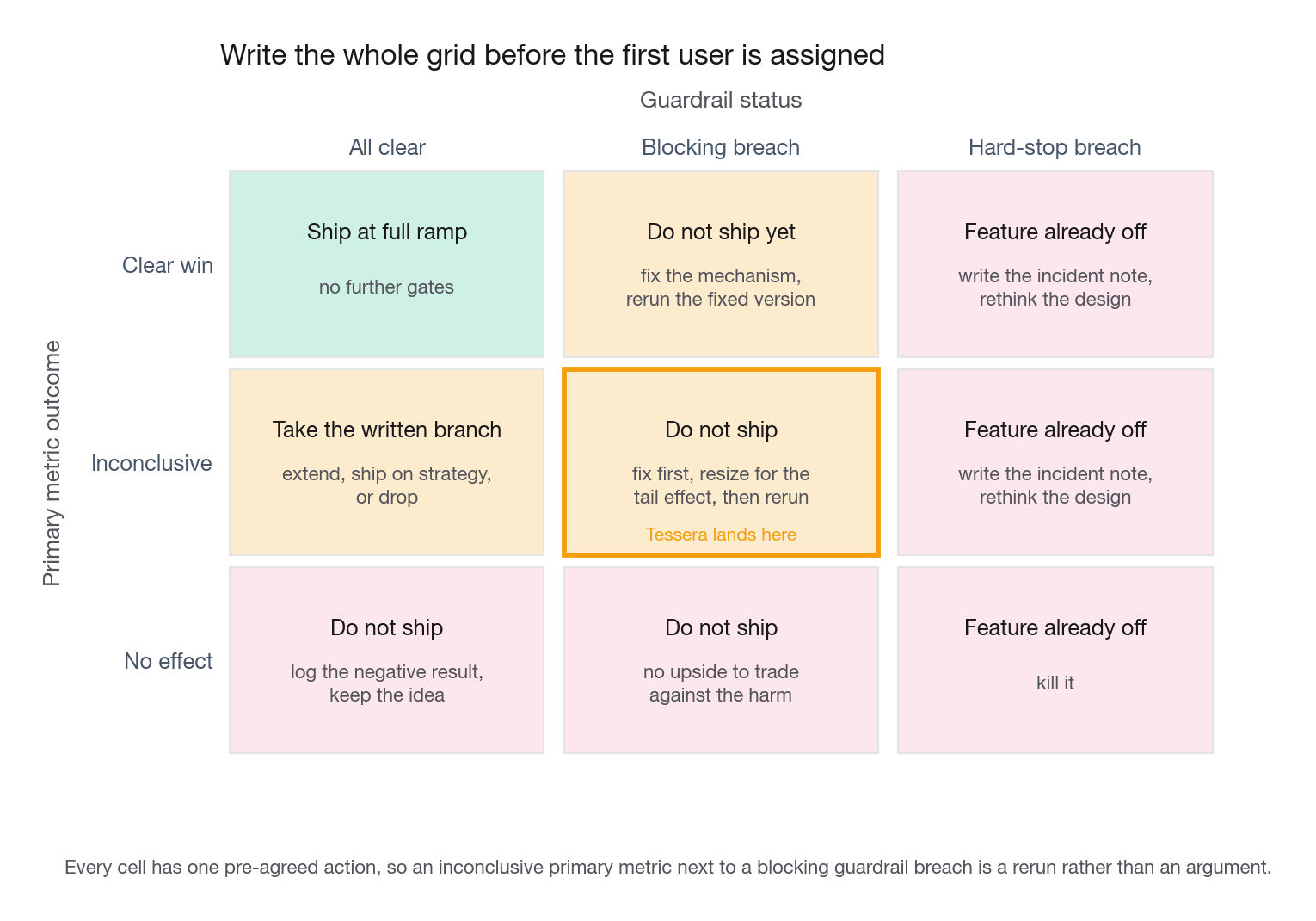
Tessera sits in the middle row, not the top: plus 1.59 percent post burn-in, interval minus 0.5 to plus 3.6, inconclusive rather than a win, next to a report-rate guardrail that could not clear its margin. Skim to the grid without that and you carry away the pooled 2.83 percent as the verdict, the exact misreading this lesson exists to prevent.
Reconstructing the exposure panel from logs
The decay analysis depends on an exposure day per user, and you almost never have that column. Build it from an exposure log joined to events.
WITH first_seen AS (
    SELECT player_id,
           variant,
           MIN(exposure_ts::date) AS first_exposure_date
    FROM   experiment_exposure
    WHERE  experiment_key = 'quick_match_v1'
    GROUP  BY player_id, variant
)
SELECT f.variant,
       (e.event_date - f.first_exposure_date) AS exposure_day,
       COUNT(DISTINCT f.player_id)            AS players,
       SUM(e.matches_started)::numeric
         / COUNT(DISTINCT f.player_id)        AS matches_per_player
FROM   first_seen f
JOIN   daily_player_activity e USING (player_id)
WHERE  e.event_date >= f.first_exposure_date
GROUP  BY 1, 2
ORDER  BY 1, 2;
Two details decide whether this is trustworthy. Use first exposure, not first assignment: a player bucketed on day 1 who does not open the app until day 6 has exposure day zero on day 6. And watch the player count per exposure day, which shrinks to the right because only early entrants have long histories. When it drops sharply, the tail of your curve describes a small self-selected group of heavy users, not the population.
Common traps
Reporting the pooled lift for a visibly new surface. The pooled 2.83 percent was nearly double the durable effect. Fix: publish the lift by exposure day next to the headline, even when it looks flat.
Slicing the trend by calendar date. That mixes users at different stages of their own adjustment, and the mix drifts as the test runs. Fix: re-index time per user before plotting decay.
Reading a subgroup null as evidence of no effect. The new-account arm could only detect about 7 percent. Fix: quote the detectable effect alongside every null.
Applying a burn-in you did not size for. Trimming a week removed about three quarters of the bias, left a residual still worth a third of the effect, and handed back an interval too wide to use. Fix: if novelty is expected, build the burn-in into the power calculation before launch.
Treating a guardrail like a second success metric. Testing a guardrail against zero blocks trivial regressions in big tests and misses serious ones in small tests. Fix: pre-register a tolerance margin and ask whether harm beyond it can be ruled out.
Setting a margin the guardrail cannot see. A margin with no power behind it blocks harmless launches: Tessera's rule would stop two in five features with a true effect of exactly zero. Fix: publish the detectable harm next to every margin at design time, and treat a straddling interval as uninformative rather than as proof of anything.
Choosing the guardrail estimand after seeing the data. The same report data gave plus 13.7 percent at p equal to 0.088 and plus 21.0 percent at p equal to 0.002, even though all three definitions are worth about 40 percent in truth. Fix: pin the aggregation in the ship rule, and for rare safety events prefer the per-player binary.
Stopping the moment the dashboard turns green. Nightly looks with a stop-on-significance rule fire falsely about one time in five. Fix: a single planned analysis, or a look schedule with widened boundaries agreed in advance.
Letting the exploratory metric wall leak into the launch memo. Two hundred uncorrected slices will hand you several exciting stories. Fix: label exploratory findings as next-experiment inputs, in writing.
No branch for inconclusive. The most common real outcome is the one nobody planned for, so it gets settled by seniority. Fix: write the third branch and name the decider before launch.
Confusing "we ran it longer" with "we removed the novelty." Averaging four weeks still blends the burst with the tail, it just downweights the burst, and trimming the early window only shrinks the blend rather than ending it. Fix: set the exclusion against a measured decay constant, or fit the decay and report its asymptote, and state the residual you kept either way.
Quick self-check
Answer each out loud in under a minute, as if the interviewer just asked.
A feature is up 6 percent after ten days. Name two diagnostics you would run first, and say what each would show if the lift were genuine rather than curiosity.
A colleague finds a change flat for accounts created after launch and up 4 percent for older ones, and calls it novelty. What single number do you ask for before accepting that, and why?
Explain to a product manager, without using the word alpha, why shipping on the first green morning is riskier than waiting for the planned end date.
A guardrail on support contacts is up 3 percent, interval minus 1 to plus 7 percent, tolerance 10 percent. Does it block the launch? Justify in terms of the margin, not the p-value.
You must report the rate of a rare safety event. Give three aggregations, say which you would pre-register, and explain what would change your mind.
Your interval covers both zero and your minimum effect, and the ship rule is silent on that case. What do you do now, and what do you change next time?