1.5 RuleFit: Turning Interactions Into Shippable Rules
Find the core decision, design, or behavior signal.
Turn the lesson into a concise response blueprint.
Name the trap you would avoid in a real interview.
Use these checkpoints as your reading path before diving into the full lesson.
- 1Why this matters in interviews
- 2Where RuleFit sits next to the other th...
- 3The dataset: Cadence picked-for-you pushes
- 4The two failures RuleFit is designed to...
- 5Failure one: the model is forced to be...
A coefficient table ranks levers. A tree shows segments. A partial dependence plot draws the shape of one lever. None of the three hands a product manager a sentence they can paste into a targeting spec. RuleFit does. This lesson is about what you reach for when an interviewer says "fine, so what do we build", and you need output written in the grammar of product logic: if this and this, then do that.
Why this matters in interviews
Product data science loops end the same way. You have described a model and what it found, and the closing question arrives: what would you ship on Monday. Weak candidates answer with a variable name. "Personalization matters, so personalize more." That is not a launch. No audience, no size, no expected lift, no way to be wrong.
The stronger answer names a population, a treatment, and a number. "Members outside Germany who listened in the last ten days, sent a brief push between 19:00 and 21:00, tap at 8.1 percent against a 4.3 percent baseline. That slice is 5.8 percent of weekly volume, about 18,400 sends, so a 15 percent relative lift clears 80 percent power in a week." There is a WHERE clause hiding in that sentence, and RuleFit writes those clauses directly instead of making you reverse engineer them from coefficients.
There is a second reason it shows up. It is the only one of the four that finds interactions and ranks them by value in the same step. A tree finds interactions but ranks them by whatever landed near one root. A regression ranks by coefficient but sees only additive terms. Interviewers asking about RuleFit are testing whether you know the regularization, not the forest, does the real work.
Interview tip: When you say "RuleFit", immediately say "so it is a lasso logistic regression whose features are the split paths of a forest". That one sentence proves you know the mechanism rather than the brand name.
Where RuleFit sits next to the other three tools
You have now seen coefficients, tree structure, and partial dependence. RuleFit is not a replacement for any of them. It occupies a specific slot: readable interactions with a value ranking attached.
| Tool | Finds | Misses | Output you can hand a PM | Cost to build |
|---|---|---|---|---|
| Logistic coefficients | Additive, monotone effects with significance | Any curvature, any interaction | A ranked lever list | Seconds |
| Single decision tree | Interactions and segments, top down | Everything the greedy first split hid; unstable | One segment definition per leaf | Seconds |
| Partial dependence | The true shape of one variable, on any model | Joint effects, unless you build 2D plots | A curve and a threshold | Minutes |
| RuleFit | Interactions, curvature, and their relative value | Anything the forest never split on | A ranked list of shippable conditions | Minutes to hours |
Read that as a sequence: coefficients to orient, a tree to test whether segmentation is the story, partial dependence to fix the shape of your continuous variables, RuleFit when the deliverable is targeting logic. If the answer is a threshold on one variable, RuleFit is overkill. If it is "these three conditions together", nothing else says so out loud.
Interview tip: If asked to pick one technique for a 45 minute case, pick coefficients plus one partial dependence plot. Reach for RuleFit only when the prompt explicitly asks for segments or targeting.
The dataset: Cadence picked-for-you pushes
Cadence is a subscription audiobook app with about 320,000 active members. Every member gets one "Picked for you" push a week suggesting a title, and growth owns how to send it better. One row is one notification, and tapped records whether the member opened the app from it within 24 hours. The frame is a 25 percent sample of one week, 80,000 rows, at a 4.3 percent base rate: the regime where accuracy is useless and log-odds arithmetic is your friend. Everything below runs against it.
| Column | Type | Meaning | Values |
|---|---|---|---|
notif_id | int | Send identifier | 1 to 80,000 |
copy_length | category | Body length variant | brief, detailed |
greeting | category | Opening line treatment | named, generic |
send_hour | int | Local hour the push went out | 6 to 22 |
weekday | category | Day of the send | Mon through Sun |
market | category | Storefront the member belongs to | US, UK, CA, AU, DE |
titles_finished | int | Lifetime completions before this send | 0 to 15 |
days_since_last_listen | int | Recency at send time, in days | 0 to 92 |
tapped | int | Opened the app within 24 hours | 0 or 1 |
Generate it once and keep it in memory.
import numpy as np
import pandas as pd

SEED = 20260826
rng = np.random.default_rng(SEED)
N = 80_000

weekdays = np.array(["Mon", "Tue", "Wed", "Thu", "Fri", "Sat", "Sun"])
markets = np.array(["US", "UK", "CA", "AU", "DE"])

copy_length = rng.choice(["brief", "detailed"], N)
greeting = rng.choice(["named", "generic"], N)
send_hour = rng.integers(6, 23, N)
weekday = rng.choice(weekdays, N, p=[.16, .16, .16, .16, .14, .11, .11])
market = rng.choice(markets, N, p=[.46, .18, .14, .12, .10])
titles_finished = rng.poisson(3.1, N)
days_since_last_listen = rng.geometric(0.11, N) - 1

z = np.full(N, -3.85, dtype=float)
z += np.where(copy_length == "brief", 0.34, 0.0)
z += np.where(greeting == "named", 0.22, 0.0)
z += np.where(np.isin(weekday, ["Sat", "Sun"]), -0.47, 0.0)
z += 0.58 * np.exp(-((send_hour - 8.5) ** 2) / 5.5)      # commute peak
z += 0.71 * np.exp(-((send_hour - 20.0) ** 2) / 6.5)     # evening peak
z += np.select([market == "DE", market == "AU"], [-0.93, -0.14], 0.0)
z += 0.31 * np.log1p(titles_finished)
z += -0.028 * np.minimum(days_since_last_listen, 45)
z += 0.86 * ((market == "DE") & (copy_length == "detailed"))          # interaction
z += 0.52 * ((days_since_last_listen > 21) & (greeting == "named"))   # interaction

notifs = pd.DataFrame({
    "notif_id": np.arange(1, N + 1),
    "copy_length": copy_length,
    "greeting": greeting,
    "send_hour": send_hour,
    "weekday": weekday,
    "market": market,
    "titles_finished": titles_finished,
    "days_since_last_listen": days_since_last_listen,
    "tapped": rng.binomial(1, 1.0 / (1.0 + np.exp(-z))),
})
Three structures are buried in there and none is visible to a plain logistic regression: the hour curve has two humps rather than a slope, the winning copy length flips inside one market, and the payoff from naming a member depends on how long they have been away. We will hand RuleFit none of the three and count how many come back. The answer is two, and the one that does not come back turns out to be the most useful part of the lesson.
The two failures RuleFit is designed to repair
Failure one: the model is forced to be monotone
Fit an unpenalized logistic regression on the raw columns and look at the send hour term.
from sklearn.linear_model import LogisticRegression

y = notifs["tapped"].values
design = pd.get_dummies(notifs.drop(columns=["notif_id", "tapped"]),
                        drop_first=True).astype(float)
flat = LogisticRegression(penalty=None, solver="lbfgs", max_iter=5000).fit(design, y)
coefs = pd.Series(flat.coef_[0], index=design.columns)
print(round(flat.intercept_[0], 4))
print(coefs[["send_hour", "days_since_last_listen", "titles_finished"]].round(4))
-3.358
send_hour 0.0142
days_since_last_listen -0.0211
titles_finished 0.0654Read that literally and the recommendation is: send later, but barely bother. Every extra hour buys about 0.014 of log-odds, so 6am to 10pm is worth roughly 0.23 in total, which most people would round to "hour does not matter much". Now look at what actually happens.
by_hour = notifs.groupby("send_hour")["tapped"].agg(sends="size", rate="mean")
by_hour["rate_pct"] = (by_hour["rate"] * 100).round(2)
print(by_hour.loc[[6, 8, 11, 14, 17, 19, 20, 22], ["sends", "rate_pct"]])
sends rate_pct
send_hour
6 4629 3.22
8 4763 5.50
11 4762 3.86
14 4810 3.12
17 4786 3.41
19 4578 6.09
20 4662 6.28
22 4601 4.87The 8am rate is 5.50 percent, the 2pm rate 3.12 percent, the 8pm rate 6.28 percent. Best hour to worst is a doubling. The linear term did not lie about the average slope: the two humps sit at opposite ends and the trough between cancels the tilt. It lied about the decision. A straight line cannot say "two windows and a dead zone", so it says almost nothing.
Now hand the regression the answer as two hand built indicators and watch what it does.
design2 = design.copy()
design2["evening"] = ((notifs["send_hour"] >= 18) & (notifs["send_hour"] <= 22)).astype(float)
design2["commute"] = ((notifs["send_hour"] >= 7) & (notifs["send_hour"] <= 9)).astype(float)
fixed = LogisticRegression(penalty=None, solver="lbfgs", max_iter=5000).fit(design2, y)
c2 = pd.Series(fixed.coef_[0], index=design2.columns)
print(c2[["send_hour", "evening", "commute"]].round(4))
send_hour -0.0104
evening 0.5377
commute 0.3462The linear term flips sign and shrinks to nothing while the indicators absorb the signal at 0.54 and 0.35. Those two numbers beat the entire original coefficient table: move a send out of the 11am to 5pm dead zone into the evening window and you gain half a unit of log-odds. Anchor that on the dead zone, not on the population average. Midday taps at 3.35 percent, so half a unit takes it to about 5.6, and the 18:00 to 22:00 block actually sits at 5.41. The raw rates put that gap at 0.50 of log-odds against the model's 0.54, so the indicator recovered the real effect to within a rounding error.
Anchoring on the 4.3 percent base instead is the mistake worth naming. That 4.3 is the average over all seventeen hours and already contains the evening hump, so adding the evening coefficient on top of it counts the hump twice and lands at 7.2 percent, higher than any hour in the table printed twenty lines ago. A converted number that beats your own best observed cell is arithmetic, not a forecast.
That is the whole idea of RuleFit in one experiment. The only thing missing is that a human picked both windows. RuleFit lets a forest propose thousands of windows and then makes a penalized regression throw away the ones that were not worth their space.
Failure two: the model cannot see interactions
The second defect is worse and less obvious. An additive model gives every member the same lift from a shorter body. Check whether that is true.
grid = (notifs.groupby(["market", "copy_length"])["tapped"].mean().unstack() * 100).round(2)
print(grid)
copy_length brief detailed
market
AU 4.48 3.19
CA 5.38 3.59
DE 2.10 3.67
UK 5.38 4.20
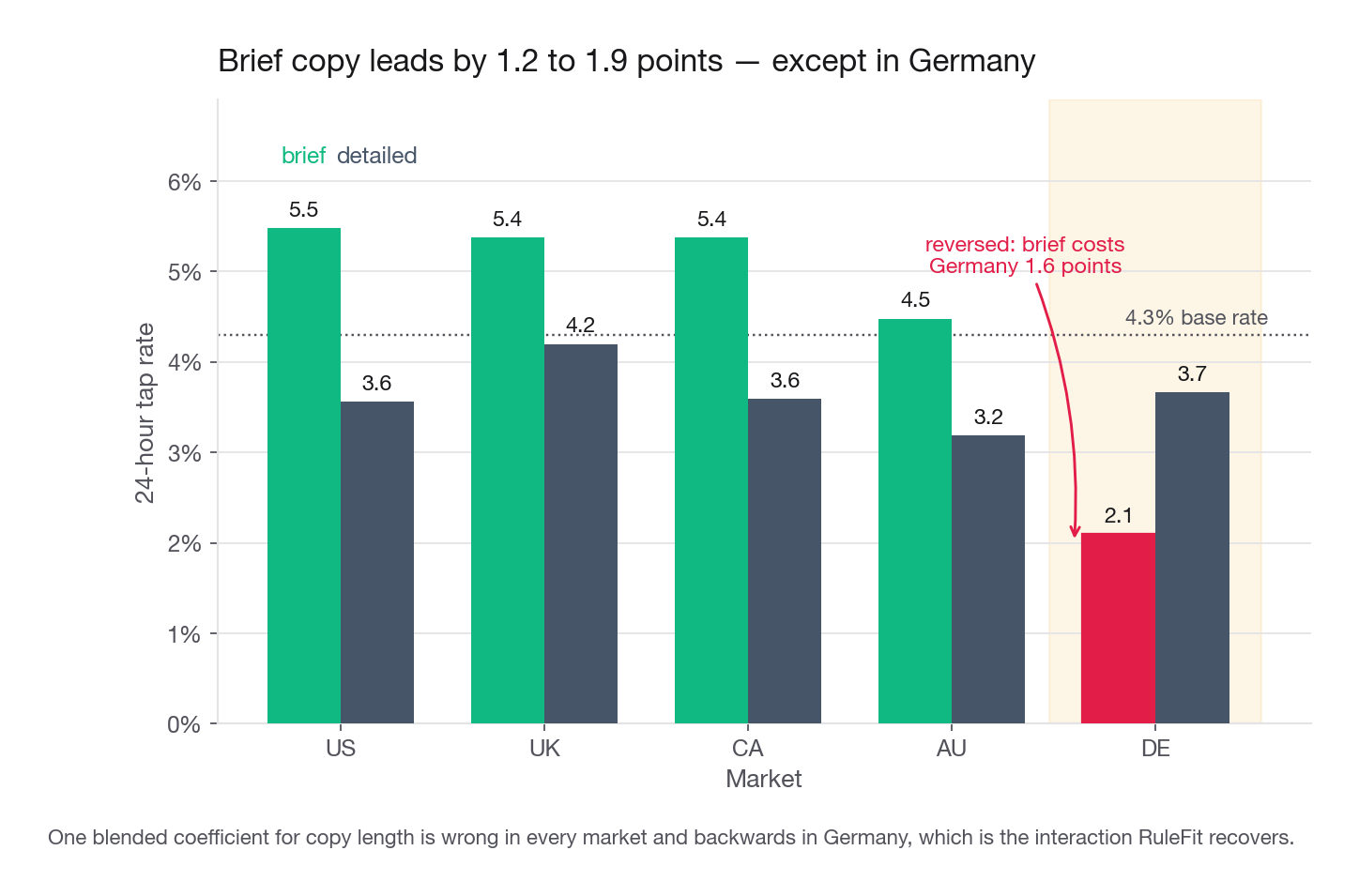
US 5.48 3.56Four markets agree that brief wins, by 1.2 to 1.9 points. Germany disagrees, and not by a rounding error: 2.10 percent for brief against 3.67 percent for detailed, the winner reversed inside 10 percent of traffic. The detailed-versus-brief log odds ratio fitted market by market reads -0.452 in the US, -0.425 in Canada, -0.353 in Australia, -0.260 in the UK, and +0.574 in Germany.
The additive model reported one blended number for copy_length_detailed, -0.327. Resist the tempting version of this argument, that the blend is wrong for everybody. It is not, and the claim collapses the moment someone checks. A pooled coefficient behaves like a precision weighted average of the strata: weight those five estimates by inverse variance and you land on -0.331, essentially the fitted value. A weighted average has to sit inside the range of the market effects, so it usually lands close to one of them. Here it lands on Australia at -0.353, a quarter of a standard error away, and it is inside about one standard error of Canada and the UK too.
What proves the model is missing something is the spread, not the misses. The estimates run from -0.452 in the US to +0.574 in Germany, a full unit of log-odds with the sign reversed at one end. Cochran's Q across the five markets is 50.4 on 4 degrees of freedom, which is not a fluctuation. Drop Germany and the remaining four are homogeneous, Q of 4.4 on 3 degrees of freedom. The US and UK gaps from the blend are sampling noise around one shared effect, not four separate failures: this copy length interaction is Germany specific and nothing else is. Read four noisy point estimates as four effects and you will build four fixes where one was needed. Standardize on brief copy everywhere and you suppress German tap rate by roughly 40 percent relative, permanently, while congratulating yourself on a global win. The same trap sits under the greeting variable.
lapsed = notifs["days_since_last_listen"] > 21
pair = (notifs.assign(lapsed=lapsed)
        .groupby(["lapsed", "greeting"])["tapped"].agg(sends="size", rate="mean"))
pair["rate_pct"] = (pair["rate"] * 100).round(2)
print(pair[["sends", "rate_pct"]])
sends rate_pct
lapsed greeting
False generic 36781 3.94
named 37069 4.88
True generic 3165 2.15
named 2985 4.22Among members who listened recently, naming them is worth 0.94 points. Among members away more than three weeks it is worth 2.07 and nearly doubles the tap rate. The blended greeting_named coefficient was 0.250; fitted separately the groups sit at 0.225 and 0.697. The lever is three times stronger exactly where you were about to write the audience off.
Interview tip: Whenever you quote a single coefficient for a treatment, add "and I checked whether that effect is constant across segments". Interviewers are listening for exactly that sentence.
How rules are harvested from an ensemble
A tree does not learn a prediction, it learns a partition, and every node in that partition is a logical statement about the data. RuleFit's insight is that those statements are reusable as features.
What counts as a rule
A rule is a path, not a leaf. If a tree splits on market = DE and then on send_hour <= 18.5, that branch yields two rules: market = DE, and market = DE AND send_hour <= 18.5. Both are real segments, and the lasso decides which earns a coefficient.
This is why a rule is a readable interaction. Nobody writes a targeting brief as "coefficient on greeting times coefficient on recency"; they write "named greeting, members away more than three weeks". A depth-3 forest produces that sentence natively, and it generates the paths before anyone decides which are interesting, which is what keeps you honest.
How many rules you get
Count the nodes. A full depth-3 tree has 2 nodes at depth 1, 4 at depth 2 and 8 at depth 3, so 14 harvestable paths per tree and 150 trees bound the library at 2,100. Trees stop early when a leaf would be too small, so the real number is 2,024 raw paths collapsing to 1,462 distinct conjunctions. That is more columns than most people have fit a regression on, out of a forest most would call too small to predict anything. Depth 6 gives 126 paths per tree, so a hundred trees is already 12,600 candidates, and depth 9 pushes past 100,000, which makes shallow the main lever on whether the pipeline finishes.
Code: walking the tree arrays
Most tutorials parse the printed text of a tree, which is fragile. Walk the arrays instead: every fitted sklearn tree exposes children_left, children_right, feature and threshold, and a recursive descent gives every path exactly once.
from sklearn.ensemble import RandomForestClassifier

X = pd.get_dummies(notifs.drop(columns=["notif_id", "tapped"])).astype(float)
names = list(X.columns)
BOOLS = {c for c in names if set(np.unique(X[c].values)) <= {0.0, 1.0}}

def harvest(est, max_conds=3):
    t = est.tree_
    paths = []
    def walk(node, conds):
        if conds:
            paths.append(tuple(conds))
        if t.children_left[node] == -1 or len(conds) >= max_conds:
            return
        f, thr = names[t.feature[node]], float(t.threshold[node])
        walk(t.children_left[node], conds + [(f, "<=", thr)])
        walk(t.children_right[node], conds + [(f, ">", thr)])
    walk(0, [])
    return paths

forest = RandomForestClassifier(n_estimators=150, max_depth=3, min_samples_leaf=500,
                                max_features=3, class_weight={0: 1, 1: 6},
                                random_state=7).fit(X, y)
raw = [r for est in forest.estimators_ for r in harvest(est)]
print(len(raw), len(set(raw)))
2024 1462The setting doing the most quiet work there is max_features=3, which forces each tree to consider only three columns per split. Without it, every tree opens on the strongest variable and the library you harvest is tiny and repetitive. Measure it rather than take my word.
import collections

roots = collections.Counter(names[e.tree_.feature[0]] for e in forest.estimators_)
print(len(roots), roots.most_common(3))

wide = RandomForestClassifier(n_estimators=150, max_depth=3, min_samples_leaf=500,
                              max_features=None, class_weight={0: 1, 1: 6},
                              random_state=7).fit(X, y)
wide_raw = [r for est in wide.estimators_ for r in harvest(est)]
wide_roots = collections.Counter(names[e.tree_.feature[0]] for e in wide.estimators_)
print(len(wide_raw), len(set(wide_raw)), len(wide_roots), wide_roots.most_common(1))
14 [('send_hour', 27), ('copy_length_detailed', 25), ('greeting_generic', 17)]
2100 306 4 [('send_hour', 138)]With column subsampling, 14 variables get a turn at the root and none opens more than 27 of the 150 trees. Without it send_hour opens 138, only four variables ever appear at a root, and 2,100 paths collapse to 306 rules. You lose four fifths of the library and every rule that exists only as a second-order combination.
Defend class_weight precisely, because the usual explanation is wrong. Six to one does not make any leaf predict a tap: at a 4.3 percent base you need about 22 to 1 before a majority vote flips, and none of the 233 leaves in the first 30 trees votes positive. The weight earns its place by reweighting impurity so rare-class purity gains count more, which changes which splits look valuable and therefore which paths exist. We collect geometry, not predictions, and Gini works happily between 2 and 8 percent without crossing 50.
Building the rule design matrix
Each harvested conjunction becomes an indicator column. Then, and this is the step most candidates forget, you filter before you fit.
PREFIX = ["copy_length", "greeting", "weekday", "market"]

def rule_mask(rule):
    m = np.ones(len(X), dtype=bool)
    for f, op, thr in rule:
        m &= (X[f].values <= thr) if op == "<=" else (X[f].values > thr)
    return m

def pretty(rule):
    out = []
    for f, op, thr in rule:
        if f in BOOLS:
            base = next(q for q in PREFIX if f.startswith(q + "_"))
            val = f[len(base) + 1:]
            out.append(f"{base} = {val}" if op == ">" else f"{base} not {val}")
        else:
            out.append(f"{f} {op} {thr:.1f}")
    return " AND ".join(out)

base_rate = y.mean()
keep, cols, seen = [], {}, set()
for rule in sorted(set(raw)):
    if sum(1 for f, op, _ in rule if op == "<=" and f in BOOLS) > 1:
        continue                       # at most one negated category, keeps rules readable
    m = rule_mask(rule)
    if not 0.03 <= m.mean() <= 0.50:
        continue                       # too rare to ship, too broad to be a segment
    if abs(np.log(y[m].mean() / base_rate)) < 0.12:
        continue                       # no marginal signal at all
    key = m.tobytes()
    if key in seen:
        continue                       # an identical column already survived
    seen.add(key)
    keep.append(rule)
    cols[rule] = m.astype(float)
print(len(keep))470From 1,462 distinct conjunctions down to 470 candidates. Four filters did that, and each is defensible in an interview.
Support floor at 3 percent. A rule covering 2,400 of 80,000 sends can carry a spectacular coefficient and still be noise. At full volume 3 percent is 9,600 sends a week, so the floor costs nothing shippable.
Support ceiling at 50 percent. A condition true for most rows is not a segment, it is a shift in the intercept. Let the linear terms carry those.
Exact-duplicate columns. Different trees rediscover the same split constantly, and two identical indicators split one coefficient arbitrarily.
Marginal signal of at least 0.12 in absolute log lift, roughly a 13 percent relative move. Not a significance test: it stops the lasso spending its budget on 400 columns sitting inside noise of the base rate.
That fourth filter has a blind spot, and it is structural rather than a tuning mistake, so it is worth understanding before it costs you something. It scores each candidate against the global base rate. Any interaction whose cell happens to sit near that base rate is therefore invisible to it, and a cell sits near the base rate exactly when a main effect and an interaction offset each other. That is not hypothetical on this dataset, and the rule table below shows which finding it costs us. The repair, when you need one, is to residualize: score the cell's observed rate against what a main effects model predicts for those same rows rather than against the global average. Here that moves the decisive candidate from a log lift of -0.08, which the gate rejects, to +0.12, which it keeps.
Interview tip: If you are asked how RuleFit avoids overfitting, do not stop at "lasso". Say support filtering first, then lasso, then a holdout check on the surviving rules. Three defenses, not one.
The L1 step: making every rule pay rent
Now fit a logistic regression on the three continuous columns plus all 470 rule columns. Standardize the continuous columns so the penalty applies on a comparable scale; the rule columns are already 0/1.
lin = X[["send_hour", "titles_finished", "days_since_last_listen"]].copy()
lin = (lin - lin.mean()) / lin.std()
R = pd.DataFrame(np.column_stack([cols[r] for r in keep]),
                 columns=[f"R{i:03d}" for i in range(len(keep))])
Z = pd.concat([lin, R], axis=1)

rulefit = LogisticRegression(penalty="l1", solver="liblinear", C=0.02,
                             max_iter=4000, random_state=0).fit(Z, y)
print(Z.shape, int((rulefit.coef_[0] != 0).sum()), round(rulefit.intercept_[0], 4))
(80000, 473) 29 -2.6859Four hundred seventy three candidates in, twenty nine out: three continuous columns and twenty six rules. That compression is the point. Note the random_state, because liblinear shuffles coordinates internally, and unpinned you get 28 terms on one run and 29 on the next and waste an afternoon hunting a phantom.
Why lasso and not ridge
Ridge shrinks every coefficient toward zero but sets none exactly to zero, so you would read 473 mostly tiny rows and the "insight" would be whatever you eyeballed. L1 puts a kink at zero in the penalty, so the optimum genuinely lands on zero for any term that does not cover its cost. The output is a subset, not a hand-thresholded ranking.
Say it in interview language: the L1 penalty makes every rule pay rent. A rule survives only if the log-likelihood it buys is larger than the penalty its coefficient costs. Rules that merely restate other rules cannot pay, because the likelihood is already bought.
Choosing C
C is the inverse penalty strength. Small C means an expensive penalty and few survivors. Sweep it and watch both sparsity and holdout performance.
from sklearn.metrics import roc_auc_score

split = np.random.default_rng(3).random(len(Z)) < 0.7
for C in [0.002, 0.005, 0.01, 0.02, 0.05, 0.1, 0.5]:
    m = LogisticRegression(penalty="l1", solver="liblinear", C=C,
                           max_iter=4000, random_state=0)
    m.fit(Z[split], y[split])
    auc = roc_auc_score(y[~split], m.decision_function(Z[~split]))
    print(C, int((m.coef_[0] != 0).sum()), round(auc, 4))
0.002 0 0.5
0.005 7 0.5948
0.01 13 0.6005
0.02 29 0.6123
0.05 44 0.617
0.1 73 0.6188
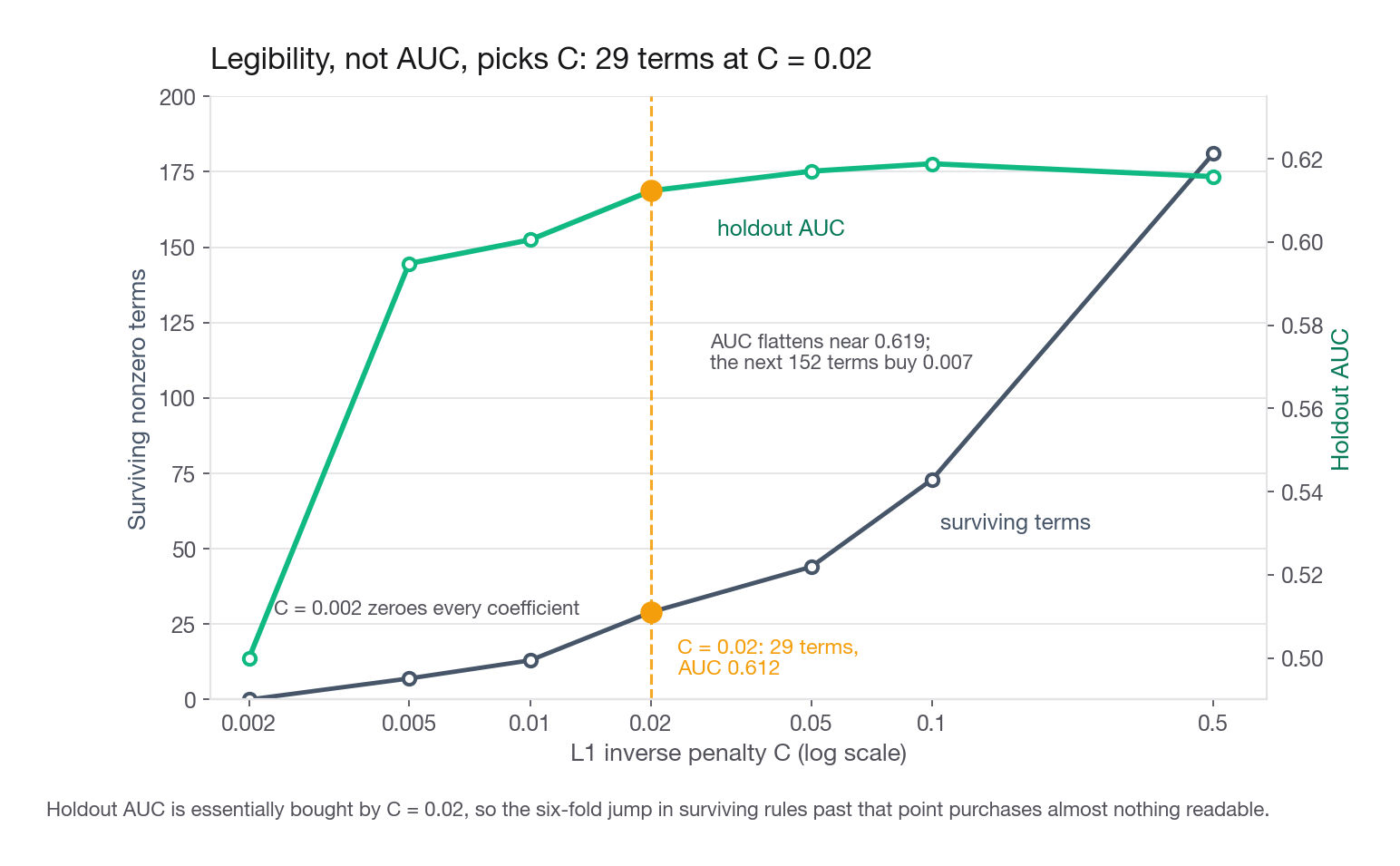
0.5 181 0.6157Read the middle of that table carefully, because it holds the argument you make out loud. Going from 44 terms to 29 costs 0.0047 of AUC. Going from 29 to 13 costs 0.0118, twice as much for a comparable term saving, and what you lose is interactions rather than main effects. So the honest operating point is C = 0.02. That trade separates "I tuned C by cross validation" from "I chose C because legibility is the objective".
One number puts the exercise in perspective. The main-effects logistic scores 0.5927 on the same holdout against the rule model's 0.6123, so 0.02 of AUC is what all this machinery bought. That is fair to poke at, and the answer is that AUC was never the deliverable: no AUC lets an additive model tell you German members want longer copy.
Reading the rule table
Pull the survivors with their coefficient, their support and their raw lift.
meta = {f"R{i:03d}": keep[i] for i in range(len(keep))}
rows = []
for term, b in zip(Z.columns, rulefit.coef_[0]):
    if b == 0 or term not in meta:
        continue
    rule = meta[term]
    m = rule_mask(rule)
    s = m.mean()
    rows.append((pretty(rule), round(b, 3), round(s, 3),
                 round(y[m].mean() / base_rate, 2),
                 round(abs(b) * np.sqrt(s * (1 - s)), 3)))
table = pd.DataFrame(rows, columns=["rule", "coef", "support", "lift", "importance"])
print(table.sort_values("importance", ascending=False).head(14).to_string(index=False))
Rewrite the raw conjunctions into product language and sort by importance, and you have the deliverable. The fitted intercept is -2.686, and the three continuous survivors are days_since_last_listen at -0.094, titles_finished at 0.084 and send_hour at 0.030, all in standardized units.
| Rule | Coefficient | Support | Raw lift | Importance |
|---|---|---|---|---|
| weekday not Mon AND weekday = Sun | -0.309 | 0.113 | 0.64 | 0.098 |
| send_hour > 10.5 AND send_hour <= 17.5 | -0.182 | 0.415 | 0.78 | 0.090 |
| send_hour > 10.5 AND send_hour <= 18.5 | -0.169 | 0.475 | 0.80 | 0.084 |
| copy_length = brief AND market = DE | -0.373 | 0.050 | 0.49 | 0.081 |
| greeting = generic AND weekday not Mon | -0.135 | 0.420 | 0.84 | 0.067 |
| copy_length = detailed AND market not UK | -0.124 | 0.412 | 0.82 | 0.061 |
| weekday = Sat | -0.140 | 0.108 | 0.78 | 0.043 |
| copy_length = brief AND days_since_last_listen <= 10.5 AND market not DE | 0.088 | 0.325 | 1.35 | 0.041 |
| copy_length = detailed AND weekday not Fri | -0.083 | 0.430 | 0.82 | 0.041 |
| copy_length not brief AND send_hour <= 18.5 | -0.080 | 0.386 | 0.75 | 0.039 |
| greeting = generic AND days_since_last_listen > 5.5 | -0.080 | 0.250 | 0.72 | 0.035 |
| greeting not named AND titles_finished <= 5.5 | -0.055 | 0.452 | 0.85 | 0.028 |
| days_since_last_listen > 8.5 | -0.049 | 0.352 | 0.80 | 0.023 |
| market not DE AND send_hour > 18.5 AND send_hour <= 21.5 | 0.062 | 0.156 | 1.43 | 0.022 |
Two of the three buried structures are there and neither was handed to the model. Row four is the German reversal, negated: brief copy into Germany carries the largest coefficient in the table, roughly double anything outside the top two. Rows two and three are the midday trough and row fourteen the evening peak, together rebuilding the shape a linear hour term destroyed.
The third, the payoff from naming a member who has been away, is missing. That miss teaches more than the two hits do.
The rule that looks like the third structure and is not
Row eleven is the trap. greeting = generic AND days_since_last_listen > 5.5 pairs exactly the two variables the interaction was planted in, carries a negative coefficient, and sits at lift 0.72, so it reads like the planted effect turned inside out. Check it before you say so in a room.
It fails on shape. The planted effect is a bonus on the NAMED arm past 21 days; row eleven is a penalty on the GENERIC arm past 5.5 days, and under 16 percent of the rows it covers are lapsed at all. Wrong arm, wrong threshold.
It fails on evidence, and this is the check to actually run. Delete the 0.52 interaction line from the generator, change nothing else, rerun the pipeline: row eleven still survives, at -0.071 against the -0.080 it earns with the interaction present. A rule keeping 89 percent of its coefficient in a world containing no interaction is not evidence of one. It is a conjunction of two negative main effects, which earns a negative coefficient whether or not anything interacts.
So here is the general rule, worth saying in these words: a conjunction is evidence of an interaction only when the matching main effects are also in the design and the conjunction still earns a coefficient. The cheap version fits one candidate at a time against saturated main effects.
me = pd.DataFrame({
    "days": np.minimum(notifs["days_since_last_listen"].values, 45).astype(float),
    "named": (notifs["greeting"] == "named").astype(float),
})
cands = {
    "named AND days > 21": ((notifs["greeting"] == "named")
                            & (notifs["days_since_last_listen"] > 21)).values,
    "generic AND days > 5.5": ((notifs["greeting"] == "generic")
                               & (notifs["days_since_last_listen"] > 5.5)).values,
}
for label, ind in cands.items():
    d = me.assign(candidate=ind.astype(float))
    fit = LogisticRegression(penalty=None, solver="lbfgs", max_iter=8000).fit(d, y)
    print(label, round(pd.Series(fit.coef_[0], index=d.columns)["candidate"], 3))
named AND days > 21 0.488
generic AND days > 5.5 -0.192With recency held saturated the planted cell earns 0.488, close to the 0.52 that went in. Row eleven earns -0.192. Rerun both against a generator with the interaction deleted and the planted cell collapses to 0.104 while row eleven barely moves, to -0.116. The first is measuring an interaction. The second is measuring two main effects standing next to each other.
Why the pipeline missed it
The forest is not at fault. It harvested days_since_last_listen > 15.5 AND greeting = named on 7.6 percent support, comfortably clear of the 3 percent floor.
The marginal signal filter is where it dies. That cell taps at 3.98 percent against a 4.315 percent base, a log lift of -0.08, so the 0.12 gate rejects it. The planted cell is no better: named AND days > 21 covers 3.73 percent of rows and taps at 4.22 percent, a log lift of -0.02. Both sit on top of the base rate because the recency main effect over 21 days is about -0.59 while the interaction is +0.52, so they nearly cancel. A filter reading marginal lift cannot see an effect that has been cancelled marginally. That is the blind spot flagged two sections ago, and this is the bill.
Loosening the filter is not enough, which is the part most people guess wrong. Drop the 0.12 gate: the candidate set grows from 470 to 663, the lapsed and named rule is in it, and the lasso zeroes it anyway at every C from 0.02 to 0.5. Hand the model the planted indicator as its own column and it is still zeroed at C = 0.02 and C = 0.05, worth 0.008 at C = 0.1, reaching 0.32 only at C = 1 where 267 terms survive and legibility is gone. The effect is real, worth about 0.49 when you ask for it directly, and this pipeline at this operating point will not pay for it.
Say that rather than rounding up to three for three. Naming the filter that dropped a finding, and why the penalty would not buy it back, beats a clean sweep, because a clean sweep on data you generated yourself is what everyone claims and nobody checks.
Coefficient, support, and importance
Three columns, three different questions.
The coefficient is a log-odds shift, as in any logistic regression, conditional on every other surviving term. Positive means the rule raises tap probability, and its size answers "how much does this move a member inside the rule".
The support is the fraction of rows where the indicator is 1. It answers "how many members does this apply to". A coefficient without support is unshippable, because a 0.09 shift over 32 percent of traffic and the same shift over 3 percent are completely different projects.
The importance multiplies the two. For a 0/1 column with support s the standard deviation is the square root of s * (1 - s), so |coefficient| * sqrt(s * (1 - s)) restates the coefficient in units of how much the feature varies. That is why the German rule, the largest coefficient in the table at -0.373, only ranks fourth: it covers 5.0 percent of sends while the rules above it cover 11 to 48 percent. Rank by importance to choose work, by coefficient to describe one member.
From log-odds to a number a PM can use
Never leave log-odds in the room. Convert.
odds0 = base_rate / (1 - base_rate)
for b in [0.088, 0.062, -0.182, -0.373]:
    p1 = 1 / (1 + np.exp(-(np.log(odds0) + b)))
    print(round(b, 3), round(np.exp(b), 3), round(100 * p1, 2))
0.088 1.092 4.69
0.062 1.064 4.58
-0.182 0.834 3.62
-0.373 0.689 3.01So the brief-and-recent rule is an odds ratio of 1.09, which at a 4.3 percent base takes a member to 4.7 percent. The midday rule costs about 0.7 points and the German brief-copy rule 1.3 points, landing at 3.0 percent. Those are sentences a PM can act on.
One caution separates a careful candidate from a fast one. Those converted numbers are what one coefficient does holding every other term at its reference. The raw segment rate is a different quantity: members outside Germany who listened within ten days and got a brief evening push tap at 8.1 percent unconditionally, not the 5.0 percent you get stacking the two positive coefficients onto the base. The gap is the negative rules, since that segment also dodges the midday trough and skews off weekends. Size experiments off the raw rate, explain levers with the coefficients, never mix them.
From a rule to shipped product logic
The technique earns its cost because surviving rules translate into code with no interpretation step. Row eight of the table is already a query.
SELECT m.member_id
FROM   members m
JOIN   push_eligibility e ON e.member_id = m.member_id
WHERE  m.market <> 'DE'
  AND  m.days_since_last_listen <= 10
  AND  e.eligible_week = DATE '2026-09-07';
Attach the treatment, brief body, named greeting, delivered between 19:00 and 21:00 local, and you have a campaign spec. Reaching it from partial dependence would take one plot per variable, a threshold call on each, and an assumption that thresholds combine additively, which is exactly what the German rule falsifies.
The holdout check is a few lines and you should never skip it.
checks = {
    "brief, recent, non-DE": ((notifs["copy_length"] == "brief")
                              & (notifs["days_since_last_listen"] <= 10)
                              & (notifs["market"] != "DE")).values,
    "brief into DE": ((notifs["copy_length"] == "brief")
                      & (notifs["market"] == "DE")).values,
}
for rule_name, target in checks.items():
    for label, sel in [("train", split), ("holdout", ~split)]:
        inside = y[sel][target[sel]]
        n, p = len(inside), inside.mean()
        print(rule_name, label, n, round(100 * p, 2), round(p / y[sel].mean(), 2),
              round(100 * np.sqrt(p * (1 - p) / n), 2))
brief, recent, non-DE train 18317 5.86 1.37 0.17
brief, recent, non-DE holdout 7694 5.68 1.28 0.26
brief into DE train 2817 1.92 0.45 0.26
brief into DE holdout 1184 2.53 0.57 0.46The targeting rule moves from lift 1.37 to 1.28 across 7,694 holdout rows. Describe that check accurately, because as written it is weaker than it looks and the description is what gets tested. Those rows were held out of one line of code and nothing else. The forest was fit on all 80,000, and every holdout row landed in the bootstrap sample of at least one of the 150 trees. The filters that cut 1,462 conjunctions to 470 both read the full-data outcome, and the model whose table you just presented was fit on all 80,000 too. So this is a split half stability check on rules chosen with knowledge of both halves, which makes it optimistic. It is still a rule you can bring to a meeting, once you have said that sentence yourself.
The German rule looks worse, 0.45 to 0.57, until you read the last column: 1,184 holdout rows carry about 30 taps at a standard error of 0.46 points on a 2.53 percent rate, so the estimates sit within one standard error. The direction is not in doubt, the magnitude is, and the right sentence is "brief copy is wrong for Germany, and I would size the test off the training estimate with a wide interval". Tolerance on a lift check is a function of positive count, not a fixed 10 percent.
The holdout that actually holds out
The honest version is about twenty lines, and running it once separates a candidate who says the word leakage from one who has measured it. Split first, then harvest, then filter, then fit, so the holdout sits outside every stage.
tr = split
forest_tr = RandomForestClassifier(n_estimators=150, max_depth=3, min_samples_leaf=500,
                                   max_features=3, class_weight={0: 1, 1: 6},
                                   random_state=7).fit(X[tr], y[tr])
raw_tr = [r for est in forest_tr.estimators_ for r in harvest(est)]
base_tr = y[tr].mean()
keep_tr, cols_tr, seen_tr = [], {}, set()
for rule in sorted(set(raw_tr)):
    if sum(1 for f, op, _ in rule if op == "<=" and f in BOOLS) > 1:
        continue
    m = rule_mask(rule)
    if not 0.03 <= m[tr].mean() <= 0.50:
        continue
    if abs(np.log(y[tr][m[tr]].mean() / base_tr)) < 0.12:
        continue
    k = m[tr].tobytes()
    if k in seen_tr:
        continue
    seen_tr.add(k)
    keep_tr.append(rule)
    cols_tr[rule] = m.astype(float)
print(len(raw_tr), len(set(raw_tr)), len(keep_tr))
1990 1468 497Standardize on training statistics too, or you leak straight back in through the scaler.
lin_tr = X[["send_hour", "titles_finished", "days_since_last_listen"]]
lin_tr = (lin_tr - lin_tr[tr].mean()) / lin_tr[tr].std()      # train statistics only
Z_tr = pd.concat([lin_tr, pd.DataFrame(np.column_stack([cols_tr[r] for r in keep_tr]),
                  columns=[f"R{i:03d}" for i in range(len(keep_tr))])], axis=1)
honest = LogisticRegression(penalty="l1", solver="liblinear", C=0.02,
                            max_iter=4000, random_state=0).fit(Z_tr[tr], y[tr])
print(int((honest.coef_[0] != 0).sum()),
      round(roc_auc_score(y[~tr], honest.decision_function(Z_tr[~tr])), 4))
21 0.6114Harvesting and filtering inside the split changes the library: 1,990 raw paths instead of 2,024, 497 candidates instead of 470, 21 surviving terms instead of 29. Holdout AUC lands at 0.6114 against the 0.6123 the contaminated pipeline reported on the same rows. The conclusion survives, and that gap of 0.0009 is what leakage of this shape is worth here. It is still real: 17 of the 470 rules kept above would have failed the signal filter on training data alone. At 80,000 rows the damage rounds away. Run the same pipeline on 8,000, where each rule covers a tenth as many positives, and it does not.
Interview tip: After presenting any rule, volunteer the sentence "this is correlational, so the ask is an experiment on this segment, not a launch". Interviewers routinely score that as a senior signal.
Overlap, redundancy, and slippery coefficients
Look again at rows two and three. The raw strings were send_hour <= 18.5 AND send_hour > 10.5 AND send_hour <= 17.5 and send_hour <= 18.5 AND send_hour > 10.5; the first collapses to an 11 to 17 window because the tighter bound wins. The forest split the same column twice in sequence and nothing simplified it. weekday not Mon AND weekday = Sun has the same shape, the first condition implied by the second.
That cosmetic redundancy is harmless once you clean the labels. The dangerous kind is different: two rules whose columns are highly correlated but not identical, so the duplicate filter misses them and the lasso splits one true effect across both by numerical accident.
surv = [t for t, b in zip(Z.columns, rulefit.coef_[0]) if b != 0 and t in meta]
corr = R[surv].corr().abs()
np.fill_diagonal(corr.values, 0.0)
shown = set()
for (a, b), v in corr.stack().sort_values(ascending=False).items():
    if tuple(sorted((a, b))) in shown:
        continue
    shown.add(tuple(sorted((a, b))))
    print(round(v, 3), "|", pretty(meta[a]), "||", pretty(meta[b]))
    if len(shown) == 3:
        break
0.927 | titles_finished <= 1.5 AND market not AU || titles_finished <= 1.5
0.886 | send_hour <= 18.5 AND send_hour > 10.5 || send_hour <= 18.5 AND send_hour > 10.5 AND send_hour <= 17.5
0.828 | days_since_last_listen > 8.5 || days_since_last_listen > 8.5 AND send_hour <= 18.5Any pair above roughly 0.85 is one finding, not two. The top pairs here are each a rule and a slightly narrower version of itself, and the -0.169 and -0.182 on the two hour windows are not two effects of that size. The consequences of ignoring overlap:
Split coefficients. One real effect of 0.30 arrives as two coefficients of about 0.15 and you undersell it by half.
Sign flips. Nested rules can give the broad rule a large positive coefficient and the narrow one inside it a large negative one. That reads as a contradiction and is only a difference. Overlapping indicators carry differences, not levels.
Fragile stories. A different forest seed reshuffles which member of a correlated pair survives, and your deck changes though the data did not.
Three fixes, in increasing order of effort.
First, collapse correlated survivors into one named segment and report the union.
Second, refit an unpenalized logistic regression on the survivors only. That takes the lasso's shrinkage off the point estimates, so a coefficient that jumps or flips sign once the penalty is gone is one whose apparent stability came from the penalty rather than the data. Then volunteer the caveat before the interviewer supplies it: the standard errors that refit prints are not valid. The same rows chose the terms and then estimated their uncertainty, so the errors run too small and the p-values are anti-conservative. That is post selection inference and there is no phrasing around it. If you genuinely need inference, select on one split and refit on a second, or reach for a selective inference method. What the refit does buy you is a redundancy diagnostic: the survivors here are 0.83 to 0.93 pairwise correlated by construction, so a standard error that explodes on a nested pair is telling you about collinearity, and that reading holds even though the p-value beside it does not.
Third, put a partial dependence plot on the fitted RuleFit model. Name this one in an interview, and name its trap in the same breath, because on a rule ensemble the obvious way to do it returns a wrong answer without complaining.
Partial dependence on a rule model needs a wrapper
rulefit was fit on Z, whose 470 rule columns are already computed. Hand Z to a partial dependence routine and it varies the standardized send_hour column while every hour rule stays frozen. The curve that comes back is a straight line spanning 0.0997 of log-odds from 6am to 10pm, numerically the same "send later, but barely bother" artifact this lesson opened by debunking, handed back with no error and no warning. To get anything real you have to rebuild the indicators from the raw features at every grid point.
lin_cols = ["send_hour", "titles_finished", "days_since_last_listen"]
lin_mean, lin_std = X[lin_cols].mean(), X[lin_cols].std()

def rule_mask_on(rule, Xraw):
    m = np.ones(len(Xraw), dtype=bool)
    for f, op, thr in rule:
        m &= (Xraw[f].values <= thr) if op == "<=" else (Xraw[f].values > thr)
    return m.astype(float)

def X_to_Z(Xraw):
    l = (Xraw[lin_cols] - lin_mean) / lin_std
    R_ = pd.DataFrame(np.column_stack([rule_mask_on(r, Xraw) for r in keep]),
                      columns=[f"R{i:03d}" for i in range(len(keep))], index=Xraw.index)
    return pd.concat([l, R_], axis=1)

obs = notifs.groupby("send_hour")["tapped"].mean()
for h in [6, 8, 14, 20, 22]:
    v = rulefit.decision_function(X_to_Z(X.assign(send_hour=float(h)))).mean()
    print(h, round(v, 3), round(100 / (1 + np.exp(-v)), 2), round(100 * obs[h], 2))
6 -3.06 4.48 3.22
8 -3.048 4.53 5.5
14 -3.361 3.35 3.12
20 -2.865 5.39 6.28
22 -2.908 5.18 4.87Even done properly it is not the double hump, and the last column is why you check rather than assume. Only four send_hour split points survive the lasso at C = 0.02, at 10.5, 17.5, 18.5 and 21.5, so the curve can only bend where those sit. It reads as a flat morning plateau near 4.5 percent, a trough near 3.3 from 11 to 5, and a peak near 5.4 from 7 to 9pm. The trough and the peak are right. The morning is not: 6am really taps at 3.22 percent and 8am at 5.50, and the plot puts both near 4.5, so the commute hump is flattened away along with the dawn dip.
That is a resolution limit rather than a blindness, and the distinction is the interesting part. The forest did split at 6.5 and 9.5, four times and twice among the distinct conjunctions, and both rules cleared the filters into the 470. C = 0.02 zeroed them, the same C chosen earlier for legibility. Push to C = 0.5 and the 6.5 split returns and the curve puts 6am at 3.23 percent against 3.22 observed. The 8am peak comes back at no C tried, because the nearest splits at 6.5 and 9.5 lump 7, 8 and 9 into one block. So the honest sentence is that a RuleFit partial dependence curve has whatever resolution your sparsity choice left it, and you should say which C the picture was drawn at.
Stability: proving a rule is real
A single fit gives one list. What you want to know is whether that list is a property of the data or of this run. Bootstrap the refit and count how often each rule survives.
sel_count = {}
boot = np.random.default_rng(11)
for _ in range(20):
    idx = boot.choice(len(Z), len(Z), replace=True)
    mb = LogisticRegression(penalty="l1", solver="liblinear", C=0.02,
                            max_iter=4000, random_state=0)
    mb.fit(Z.iloc[idx], y[idx])
    for term, b in zip(Z.columns, mb.coef_[0]):
        if b != 0:
            sel_count[term] = sel_count.get(term, 0) + 1
freq = pd.Series(sel_count).sort_values(ascending=False) / 20
for term, f in freq.head(12).items():
    print(round(f, 2), pretty(meta[term]) if term in meta else term)
1.0 titles_finished
1.0 copy_length = brief AND market = DE
1.0 send_hour <= 18.5 AND send_hour > 10.5 AND send_hour <= 17.5
1.0 weekday not Mon AND weekday = Sun
1.0 greeting = generic AND weekday not Mon
1.0 days_since_last_listen
0.95 send_hour <= 18.5 AND send_hour > 10.5
0.95 weekday = Sat
0.9 copy_length = detailed AND market not UK
0.9 copy_length = detailed AND weekday not Fri
0.75 send_hour
0.7 titles_finished <= 1.5 AND market not AUThe German rule survives all 20 resamples on 5 percent support, which answers anyone assuming small support means unstable. Small support widens the lift interval; it does not make the rule optional. The linear send_hour term appears in only 15 of 20, which is exactly right: once the window rules exist, the straight line has nothing left to explain.
| Selection frequency | Interpretation | What to do with it |
|---|---|---|
| 0.95 to 1.00 | Structural. Present in essentially every resample | Put it in the deck; design the experiment around it |
| 0.70 to 0.94 | Probably real but entangled with a correlated sibling | Merge with the sibling, or report as one segment |
| 0.40 to 0.69 | Sensitive to sample; often a narrower slice of a stable rule | Mention only as supporting texture, never as a headline |
| Below 0.40 | Noise the penalty happened to spare in one fit | Drop it, and do not let it into the slides at all |
Two extra checks are cheap. Refit the whole pipeline with a new forest seed, not just a bootstrap of the regression, since instability can live in the harvest. And recompute support and lift for every headline rule on a time based holdout, since a rule holding only in older data describes a product that no longer exists.
Cost, and when not to reach for RuleFit
The four stages run strictly in sequence: no harvest before the forest, no binarization before the rules, no lasso before the matrix. Wall clock time is their sum and all four scale with forest size, so doubling the trees doubles everything.
This matters for insight quality, not patience. Tuning is iterative, and a pipeline taking two hours per run gets tuned twice rather than twenty times. Under tuned models give mushy rules, and mushy rules give recommendations that die in their first experiment. Two hundred shallow trees is not a compromise, it is what makes the loop converge.
One honest limitation: RuleFit never went mainstream, so tooling is thin and you debug breakages yourself. That is a fair answer if an interviewer asks why you would skip it. It also argues for rolling your own, as here: harvest plus lasso is forty lines and gives you exact control over the support filter, the length cap and the negation policy.
Common traps
Reporting rules without support. A coefficient of 0.9 on 0.4 percent of traffic is a curiosity. Print support beside every coefficient and set the floor before you fit.
Treating overlapping coefficients as independent effects. When two rules nest, as the hour windows do here, their coefficients are a level and a difference, not two levels. Merge correlated survivors, and use partial dependence for a variable's net effect, remembering that on a rule model that means mapping raw features back through the rule transform rather than handing the rule matrix to a partial dependence routine.
Reading a conjunction as an interaction. Two variables sharing one rule proves nothing by itself, because a conjunction of two negative main effects earns a negative coefficient in a world with no interaction in it. Refit the candidate against saturated main effects before you call it an interaction.
Letting every tree see every column. The default
max_featurescollapsed the library from 1,462 rules to 306 and let one variable open 138 of 150 trees. Subsample or you harvest the same rule repeatedly.Growing a deep forest because it predicts better. Depth 6 gives six-condition rules nobody will implement covering a handful of rows. Cap depth at 2 or 3 and cap rule length in the harvest.
Forgetting to standardize the continuous terms. L1 is scale sensitive. With
days_since_last_listenrunning 0 to 92 against 0/1 rules the penalty falls unevenly, and you conclude recency did not matter.Leaving the solver unseeded. liblinear shuffles coordinates, so an unpinned fit changes its survivor count run to run.
Presenting raw machine generated strings.
weekday not Mon AND weekday = Sunsays you did not read your own output. Simplify, rename into product language, sort by importance.Claiming causality. Every rule here is a conditional association in observational send data. RuleFit outputs a hypothesis with an audience attached; the next artifact is a test plan.
Tuning C by AUC alone. The best AUC here buys 0.0065 for 44 extra terms. Take the sparsest model within a small tolerance of the best, because the deliverable is a readable list.
Quick self-check
Answer these out loud, in full sentences, as if the interviewer just asked.
Explain RuleFit in three sentences without reusing the word after the first one. Name the forest, the binarized paths, and the L1 penalty, and say what the penalty buys.
The linear
send_hourcoefficient came out at 0.014 while the best hour taps at twice the worst. Explain how both are true, and what you would have shipped on the coefficient alone.Your top rule has coefficient 0.31 on support 0.05, another 0.09 on support 0.42. Which do you work on first, and what quantity are you comparing?
A rule reads
send_hour > 10.5 AND send_hour <= 17.5at -0.182 and a broadersend_hour > 10.5 AND send_hour <= 18.5at -0.169. What does the first coefficient measure, and what would you wrongly conclude reading it alone?Base tap rate is 4.3 percent and a rule has coefficient -0.373 on 5 percent of sends. Convert to an odds ratio and an absolute probability, then give the one line PM summary and say why you would not launch yet.
You rerun the pipeline with a new forest seed and half the rules change. Name three things you check, in order, before deciding whether the original findings hold.