2.4 Short-Term Wins Versus Long-Term Health
Find the core decision, design, or behavior signal.
Turn the lesson into a concise response blueprint.
Name the trap you would avoid in a real interview.
Use these checkpoints as your reading path before diving into the full lesson.
- 1Why this matters in interviews
- 2The shape of the trade
- 3Renewable versus non-renewable levers
- 4The one-line diagnostic
- 5A dataset to make this concrete
Some changes make a number go up this week by quietly spending something you will need next year. Heavier ad load, more push notifications, an aggressive first-order discount, a ranking model tuned on clicks: each of them buys a real gain today with a real cost that arrives after the test has been called a success. This lesson gives you the machinery to spot that shape, price it, measure it in a window shorter than the damage takes to appear, and then win the argument for shipping a change that loses money for a quarter.
Why this matters in interviews
The interviewer almost never asks "is this a short-term versus long-term tradeoff." They hand you a prompt where the tradeoff is buried and watch whether you find it. Three real openers:
"We ran a test that increased ads per session from three to four. Revenue per user went up eleven percent, the result was significant, retention showed no significant difference. Do we ship it?"
"Growth wants to double push notification volume. What would you want to see before you agree?"
"One advertiser has by far the best click rate on our network. How would you tell whether that is good news?"
Every one has the same skeleton: a lever raises yield per unit of exposure and, on a delay, shrinks the base of exposures. The candidate who says "revenue is up eleven percent and retention is flat, ship it" has answered a question about a two week window nobody cares about. The candidate who says "flat retention over two weeks is what a retention effect looks like before it shows up, here is how long I would need and what I would watch instead" is doing the job.
There are four scoreable moves, and they are what the rest of this lesson drills:
Name the borrowed resource. What exactly is being spent, and does it regenerate.
Convert both sides into one currency, which is almost always discounted contribution per user over a stated horizon.
Find something observable inside the test window that predicts the part you cannot wait for.
Commit, in advance, to a decision rule and a long-run measurement that will still be running after everyone has moved on.
Interview tip: When a prompt reports a positive result with "and retention was flat," treat that as the interesting sentence, not the reassuring one: ask first how long users were followed, because a retention number nobody waited for is censored rather than null, and only then what effect size the test could actually resolve.
The shape of the trade
Start by writing the metric as an identity. For an ad-supported product:
weekly revenue = active users x sessions per active user x ads per session x click rate x revenue per click
Raising ads per session multiplies one term by 4/3. Nothing in the identity says the other terms hold still. In practice two of them respond, on different clocks:
Click rate drops almost immediately, because the fourth ad in a session is seen with less attention than the third. This shows up inside days.
Active users and sessions per active user drop slowly, because annoyance accumulates and quitting an app is a decision people make once, at a moment that has nothing to do with the week the change shipped.
That gap in clocks is the whole problem: the fast terms are the ones the change was designed to move, and the slow ones are what pays for it.
Renewable versus non-renewable levers
Not every borrow is equally dangerous, and this distinction is the fastest way to sound senior. Some levers deplete something that grows back if you stop. Others spend something you cannot get back at any price.
| Lever | What it borrows | Regenerates if you stop | Typical lag to visible cost |
|---|---|---|---|
| Ads per session up 33 percent | Session tolerance, attention | Mostly yes, over weeks | 6 to 14 weeks |
| Push notifications up 2x | System-level notification permission | No, opt-out is one-way | 1 to 3 weeks for opt-out, months for the session loss |
| Interstitial on app open | Cold-start patience | Partly | 2 to 8 weeks |
| First-order discount of 40 percent | Reference price, margin expectation | No, the anchor persists | 1 to 2 purchase cycles |
| Ranking tuned purely on clicks | Trust that the feed is worth opening | Slowly and incompletely | 8 to 20 weeks |
| Emailing lapsed users weekly | Deliverability reputation | No, domain reputation is sticky | 3 to 12 weeks |
The right-hand pattern matters more than the exact numbers. When the borrowed resource does not regenerate, a reversible experiment is a lie: you can turn the treatment off, but users who revoked notification permission do not come back. That means you cannot learn cheaply by shipping and watching.
Interview tip: Say the words "this is a one-way door for notification permission, so I want the decision made before the launch, not after" and you have separated yourself from every candidate who proposed shipping and monitoring.
The one-line diagnostic
For any prompt, ask which large term in the identity the change does not touch directly, and by what mechanism it responds. Name a mechanism and you have a hypothesis worth measuring. Fail to name one and the change is probably a genuine free win, which you should say rather than manufacture a concern. Reflexively finding a dark side in every idea reads as contrarian, not rigorous.
A dataset to make this concrete
The running example is Nightjar, a mobile long-form audio app monetized with in-stream audio ads. The product team ran a 13 week experiment that raised ad load from three to four spots per session. The block below regenerates the user-week panel deterministically so every number later in this lesson is reproducible.
import numpy as np
import pandas as pd

SEED = 41072026
rng = np.random.default_rng(SEED)

N_USERS, WEEKS = 40_000, 13
CPC_USD, ADS_CONTROL, ADS_HEAVY = 0.42, 3.0, 4.0

arm = rng.choice(["control", "heavy_ads"], size=N_USERS)
heavy = (arm == "heavy_ads")
base_sessions = 0.4 + rng.gamma(2.2, 1.7, size=N_USERS)

alive, rows = np.ones(N_USERS, dtype=bool), []
for w in range(1, WEEKS + 1):
    ads = np.where(heavy, ADS_HEAVY, ADS_CONTROL)
    ctr = np.where(heavy, 0.0185, 0.0210)
    sessions = np.where(alive, rng.poisson(base_sessions), 0)
    impressions = (sessions * ads).astype(int)
    clicks = rng.binomial(impressions, ctr)
    rows.append(pd.DataFrame({
        "user_id": np.arange(N_USERS), "arm": arm, "week": w,
        "active": alive.astype(int), "sessions": sessions,
        "impressions": impressions, "clicks": clicks,
        "revenue_usd": clicks * CPC_USD,
    }))
    alive = alive & (rng.random(N_USERS) > 0.030 + 0.0018 * w * heavy)

panel = pd.concat(rows, ignore_index=True)
The generator encodes the structure described above: a third more inventory, a slightly worse click rate per spot, and a churn hazard that starts identical and drifts upward with cumulative exposure. Nobody hands you a dataset with the mechanism labelled; the point of building one is to check whether your reading procedure would have caught it.
Reading the experiment honestly
The naive read
Compute revenue per assigned user and survival per arm. Always divide by users assigned, never by users still active, or you have conditioned on an outcome the treatment causes.
size = panel.groupby("arm")["user_id"].nunique()
rev_pu = panel.groupby(["arm", "week"])["revenue_usd"].sum().unstack(0).div(size, axis=1)
surv = panel.groupby(["arm", "week"])["active"].sum().unstack(0).div(size, axis=1)

read = rev_pu.assign(lift=rev_pu["heavy_ads"] / rev_pu["control"] - 1)
print(read.round(4))
print(surv.round(4))
arm control heavy_ads lift
week
1 0.1103 0.1302 0.1808
2 0.1051 0.1256 0.1952
3 0.1031 0.1179 0.1440
4 0.0990 0.1134 0.1451
5 0.0968 0.1088 0.1240
6 0.0920 0.1080 0.1732
7 0.0902 0.1049 0.1639
8 0.0899 0.1000 0.1121
9 0.0842 0.0949 0.1270
10 0.0820 0.0901 0.0982
11 0.0823 0.0857 0.0404
12 0.0781 0.0814 0.0419
13 0.0735 0.0765 0.0408
arm control heavy_ads
week
1 1.0000 1.0000
2 0.9691 0.9673
3 0.9391 0.9356
4 0.9110 0.9019
5 0.8844 0.8697
6 0.8584 0.8351
7 0.8337 0.7993
8 0.8095 0.7643
9 0.7858 0.7306
10 0.7629 0.6950
11 0.7381 0.6614
12 0.7174 0.6297
13 0.6955 0.5961If your team called the test at two weeks, which is what most teams do, the readout was a 19 percent revenue lift with no visible retention effect. Ship it, write the doc, take the win.
The read that changes your mind
Two things in that table should stop you. The lift is trending down, from 18 percent in week one to 4 percent in week thirteen, and the survival curves have separated by ten points. Note the word trending: on 20,000 users per arm the weekly lift rises in five of its twelve transitions, including 4.9 points from week five to week six. The path underneath is monotone, 17.5 percent falling to 1.5 percent on the generator's own parameters, but no thirteen week readout at this size marches down in a straight line, and narrating the wiggles is reading noise.
cum = rev_pu.cumsum()
print("13-week revenue per assigned user:", cum.iloc[-1].round(4).to_dict())
print("cumulative lift:", round(cum.iloc[-1]["heavy_ads"] / cum.iloc[-1]["control"] - 1, 4))
print("retention gap (pp):", round((surv.iloc[-1]["control"] - surv.iloc[-1]["heavy_ads"]) * 100, 2))
13-week revenue per assigned user: {'control': 1.1867, 'heavy_ads': 1.3375}
cumulative lift: 0.1271
retention gap (pp): 9.95Here is the uncomfortable part, and it is the reason this lesson exists. After a full quarter, the cumulative revenue readout is still positive: plus 12.7 percent. There is no week in the test where the treated arm's weekly revenue falls below control. Every dashboard in the company says this worked. And it is still, as the next section shows, a wash at a one year horizon and clearly destructive beyond that.
That is the thing to internalise about this class of change. The failure mode is not that the test turns negative and someone ignores it. It is that the test never turns negative inside any window a company will wait, because the loss is carried by a shrinking base whose absence compounds after the experiment is shut off.
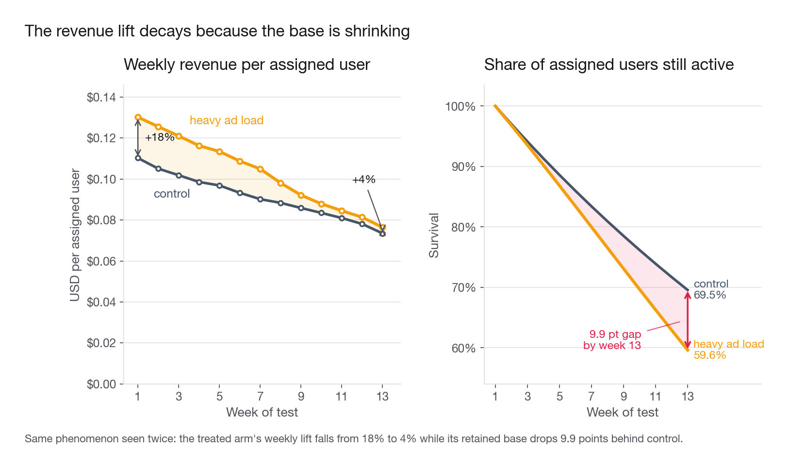
Interview tip: State explicitly that a decaying treatment effect and a widening survival gap are the same phenomenon seen twice, because revenue per assigned user equals revenue per active user times survival, and here the per-active ratio sits flat around 1.18 for all thirteen weeks while the survival ratio falls from 1.00 to 0.857.
Compute that decomposition rather than asserting it, because the tempting explanation is a different one and it is wrong here. The tempting story is compositional: the treated arm sheds its least tolerant users first, so the survivors are a tougher crowd. Check the direction before you say it. If that were happening the treated survivors would get steadily more tolerant, revenue per active user in the treated arm would drift up, and the effect would offset the decay rather than cause it. Nightjar has no such heterogeneity, every treated user carries the same hazard of 0.030 plus 0.0018 times the week, and the panel agrees: the heavy arm earns 0.1302 per active user in week one and 0.1284 in week thirteen, against a mechanical 4 times 0.0185 over 3 times 0.0210. So the entire decay is the shrinking denominator. This is the moment to say "that pattern is consistent with selective attrition but does not demonstrate it, and here is the plot that separates them," rather than reaching for the more interesting mechanism. The plot is revenue per active user by arm: flat means no compositional shift, a rising treated line means selective attrition. Use it to decompose only, because the number you report still divides by assigned users.
Lifetime value as the arbiter
You cannot compare "plus 12.7 percent revenue this quarter" against "ten fewer retained users per hundred" until both are in one currency. That currency is lifetime value.
Define it so two people compute the same number
Most candidates say "lifetime value" and stop. A usable definition needs five decisions, and interviewers who work on monetization will probe all five.
| Decision | Weak default | What to say instead |
|---|---|---|
| Numerator | Revenue | Contribution margin, revenue minus variable serving, payment, support, and content cost |
| Horizon | "Lifetime" | A stated finite horizon, 12 or 24 months, chosen to match the decision |
| Discounting | None | A weekly rate derived from the company's cost of capital |
| Population | Users who converted | Everyone assigned or acquired, including the ones worth zero |
| Survival | Assumed constant | Estimated from the tail of the observed curve, and stated as an assumption |
For Nightjar the variable cost is content licensing plus delivery, roughly 0.045 USD per active user-week. Ad revenue is high margin but not free.
VAR_COST = 0.045
tail = surv.iloc[-5:]
hazard = 1 - (tail.iloc[-1] / tail.iloc[0]) ** (1 / 4)
margin = rev_pu.iloc[-1] / surv.iloc[-1] - VAR_COST
banked = rev_pu.sum() - VAR_COST * surv.sum()

print("weekly churn hazard:", hazard.round(4).to_dict())
print("contribution per active user-week:", margin.round(4).to_dict())
print("banked contribution per assigned user:", banked.round(4).to_dict())
weekly churn hazard: {'control': 0.03, 'heavy_ads': 0.0496}
contribution per active user-week: {'control': 0.0607, 'heavy_ads': 0.0834}
banked contribution per assigned user: {'control': 0.696, 'heavy_ads': 0.8702}So the test window banked an extra 0.174 USD of contribution per assigned user, and left the treated arm with a weekly churn hazard of 4.96 percent against 3.00 percent. Those two numbers are the whole decision.
Estimating lifetime value: four methods that answer different questions
Interviewers like to ask "how would you estimate it," and the good answer is a question back: estimate it for what. The method follows the use.
| Method | How it works | Best for | Fails when |
|---|---|---|---|
| Historical cohort | Take cohorts old enough to have aged a full horizon, sum realised margin | Board-level reporting, sanity checks | The product changed; you are measuring an app that no longer exists |
| Survival times margin | Fit a churn hazard, multiply by contribution per active period, discount | Experiment arbitration, this lesson's use | Hazard is not flat and your tail is short |
| Predictive model at acquisition | Supervised model on features known at first visit, target is horizon margin | Bidding, channel budgets, welcome-offer sizing | Trained on year-old cohorts that no longer resemble today's traffic |
| Contractual or subscription DCF | Known price times modelled renewal, discounted | Subscription products with explicit terms | Non-contractual products where nobody ever formally cancels |
For an ad-load decision you want method two, because it isolates the mechanism you changed. For the question below you want method three.
The first-session model, at Portside Goods
Switch products for a moment, because interviewers love this variant. Portside Goods is a home-textiles marketplace. The question: a visitor lands on the homepage for the first time and has not bought anything. What is that visitor worth?
Frame it as supervised regression on a horizon-bounded target: discounted contribution over the 12 months after the first visit, trained on visitors whose first visit was at least 13 months ago so every label is complete. Use only features available at prediction time: acquisition channel, the query that produced the click and its commercial-intent bucket, brand against category ad, device class and operating system, browser locale as a language proxy, country and metro, and calendar week, which carries real signal because a first visit in mid-November is worth far more than the same visit in February.
Two structural points that separate a good answer from a recital:
Model the zero. Most first-time visitors never buy. A single regression on a target that is zero 92 percent of the time will fit the zeros and shrink everything else toward them. Either use a two-part model, one classifier for "buys within 12 months" and one regression for margin conditional on buying, or use a loss designed for non-negative skewed targets such as Tweedie. State which and why.
Predict the segment, not the person. The output is almost never used per user. It is used to set an acquisition bid, a welcome-offer size, or a channel budget, all of which are decisions made over groups. That means you need calibrated conditional means for segments, not sharp individual ranking, and it makes a shallow tree genuinely useful because its leaves are the segments and the leaf means are the bids.
# Sketch: two-part first-session value model for Portside Goods.
# X_train, X_new are yours; y_train is 12-month contribution, zero for non-buyers.
from sklearn.ensemble import HistGradientBoostingClassifier, HistGradientBoostingRegressor

buyer = HistGradientBoostingClassifier(max_depth=4).fit(X_train, y_train > 0)
size = HistGradientBoostingRegressor(loss="gamma", max_depth=4)
size.fit(X_train[y_train > 0], y_train[y_train > 0])

expected_value = buyer.predict_proba(X_new)[:, 1] * size.predict(X_new)
The loss on the size model is load-bearing, and interviewers catch people here. The decomposition only multiplies through for means: expected value is probability of buying times the mean margin among buyers. A quantile loss such as absolute_error returns the conditional median, and order values are skewed enough that the median sits well below the mean. On a two-part simulation with 91 percent zeros and a lognormal positive part, absolute_error recovers 0.86 of the true mean at mild skew and 0.53 at heavy skew, against about 1.02 for the default squared_error and 0.98 down to 0.88 for gamma. The bias runs one way and is worst where the tail is fattest, so when dispersion differs across channels the median version can rank channels backwards. Prefer gamma for a money target: the size model is already fit only on positive labels, and unlike poisson it does not force variance to equal the mean. Tweedie is the single-model alternative fit on every row including the zeros, not a swap for the size model, and in scikit-learn that means TweedieRegressor, not HistGradientBoostingRegressor, which has no tweedie loss.
The trap nobody mentions unprompted: your labels are 13 months stale by construction, so the model has learned last year's checkout flow, last year's shipping speeds, and last year's competitor set. Say out loud how you would handle it. The standard fix is to train on complete labels but recalibrate on recent cohorts using an early surrogate, which is exactly the proxy machinery two sections down.
Interview tip: For any lifetime value question, name the horizon and the margin definition in your first two sentences, before any modelling talk, because those two choices move the answer more than the model class ever will.
Horizon and discounting decide the answer
Now price the Nightjar decision. Banked contribution is known. Forward contribution is a discounted sum over the surviving base.
def forward_value(margin, hazard, alive, horizon, annual_discount=0.12):
    d = (1 + annual_discount) ** (1 / 52) - 1
    f = (1 - hazard) / (1 + d)
    return alive * margin * f * (1 - f ** horizon) / (1 - f)

for H in (13, 26, 52, 104):
    fwd = {a: forward_value(margin[a], hazard[a], surv.iloc[-1][a], H)
           for a in ("control", "heavy_ads")}
    delta_fwd = fwd["heavy_ads"] - fwd["control"]
    total = (banked["heavy_ads"] - banked["control"]) + delta_fwd
    print(H, round(delta_fwd, 4), round(total, 4))
13 0.0145 0.1887
26 -0.0451 0.1291
52 -0.1845 -0.0103
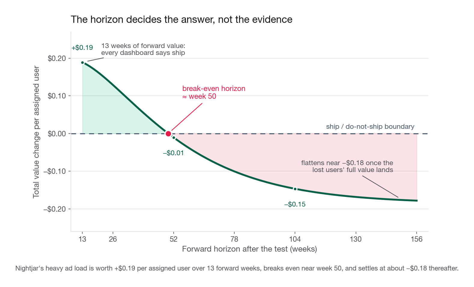
104 -0.3202 -0.1461Read that as a table, because it is the punchline of the lesson.
| Forward horizon after the test | Change in forward value per assigned user | Total value change per assigned user | 95 percent interval on the total | Decision |
|---|---|---|---|---|
| 13 weeks | +0.0145 USD | +0.189 USD | +0.139 to +0.241 | Ship, confidently |
| 26 weeks | -0.045 USD | +0.129 USD | +0.056 to +0.204 | Ship |
| 52 weeks | -0.185 USD | -0.010 USD | -0.111 to +0.093 | Coin flip |
| 104 weeks | -0.320 USD | -0.146 USD | -0.265 to -0.023 | Do not ship |
Intervals come from the user-level bootstrap at the end of this section. Add them before anyone asks: they change no label, and they are what makes "coin flip" a measurement rather than a turn of phrase.
The same experiment, the same data, four different answers. Nothing about the evidence changed. Only the horizon did.
This is why the horizon is not an implementation detail you can leave to the analyst. It is the decision. Choose it before you see the result, and choose it on a principle you can defend: match it to the payback period the finance team already uses for customer acquisition, or to the planning cycle the decision belongs to. If your company pays back paid acquisition in 9 months, evaluating product changes on a 13 week horizon means product is allowed to destroy value that marketing is not.
Discounting, briefly and correctly
The rate does less work than people expect. At 12 percent annual the weekly rate is about 0.218 percent, and over 52 weeks it shaves the forward term by roughly 6 percent; doubling it to 24 percent flips no row in the table above. Do not spend interview time arguing 10 against 15. Spend it on the horizon and the hazard estimate, which are worth ten times more. The rate matters mainly at a startup, where the honest discount is the return on the next dollar of runway rather than a textbook cost of capital.
Turn it into a break-even, which is the version that survives disagreement
Nobody will agree with your hazard estimate. Rather than defending it, invert the question: how much extra churn would the change have to cause before it stops being worth it.
lo, hi = 0.0, 0.10
for _ in range(50):
    mid = (lo + hi) / 2
    fwd_h = forward_value(margin["heavy_ads"], hazard["control"] + mid,
                          surv.iloc[-1]["heavy_ads"], 52)
    fwd_c = forward_value(margin["control"], hazard["control"],
                          surv.iloc[-1]["control"], 52)
    if (banked["heavy_ads"] - banked["control"]) + (fwd_h - fwd_c) > 0:
        lo = mid
    else:
        hi = mid

print("break-even incremental weekly hazard:", round(lo, 4))
print("observed incremental weekly hazard:", round(hazard["heavy_ads"] - hazard["control"], 4))
break-even incremental weekly hazard: 0.0189
observed incremental weekly hazard: 0.0196The change breaks even at 1.89 points of extra weekly churn and the data says 1.96. Now the meeting is about one number that everyone can attack, which is exactly where you want it. If someone believes the true incremental hazard is 1.5 points, they have made a falsifiable claim and you can go measure it.
What you cannot do is stop there and declare the argument over, because a 0.07 point gap between an estimate and a threshold is not a result. Both sides come from the same 40,000 users, so both carry sampling error, and the threshold is the wider one. Resample users with replacement and push each replicate through the whole pipeline.
BOOT, brng = 2000, np.random.default_rng(902)
rev_m = panel.pivot_table(index="user_id", columns="week", values="revenue_usd").values
act_m = panel.pivot_table(index="user_id", columns="week", values="active").values
hv = panel.sort_values("user_id").groupby("user_id")["arm"].first().values == "heavy_ads"

def arm_stats(rev, act, m):
    rp, sv = rev[m].sum(0) / m.sum(), act[m].sum(0) / m.sum()
    return (1 - (sv[-1] / sv[-5]) ** 0.25, rp[-1] / sv[-1] - VAR_COST,
            rp.sum() - VAR_COST * sv.sum(), sv[-1])

def replicate(i):
    c, t = arm_stats(rev_m[i], act_m[i], ~hv[i]), arm_stats(rev_m[i], act_m[i], hv[i])
    net = lambda extra, H: (t[2] - c[2]) + forward_value(t[1], c[0] + extra, t[3], H) \
                                         - forward_value(c[1], c[0], c[3], H)
    lo, hi = 0.0, 0.10
    for _ in range(50):
        mid = (lo + hi) / 2
        lo, hi = (mid, hi) if net(mid, 52) > 0 else (lo, mid)
    obs = t[0] - c[0]
    return [obs * 100, lo * 100] + [net(obs, H) for H in (13, 26, 52, 104)]

boot = np.array([replicate(brng.integers(0, len(hv), len(hv))) for _ in range(BOOT)])
q = lambda a, k=2: np.percentile(a, [2.5, 97.5]).round(k)

print("incremental hazard (pp):", boot[:, 0].mean().round(2), q(boot[:, 0]))
print("break-even hazard (pp):", boot[:, 1].mean().round(2), q(boot[:, 1]))
print("gap (pp):", (boot[:, 0] - boot[:, 1]).mean().round(2), q(boot[:, 0] - boot[:, 1]))
for k, H in enumerate((13, 26, 52, 104), start=2):
    print(H, "weeks:", boot[:, k].mean().round(3), q(boot[:, k], 3),
          "P(>0) =", round((boot[:, k] > 0).mean(), 2))
incremental hazard (pp): 1.96 [1.74 2.19]
break-even hazard (pp): 1.9 [1.29 2.58]
gap (pp): 0.06 [-0.69 0.74]
13 weeks: 0.189 [0.139 0.241] P(>0) = 1.0
26 weeks: 0.129 [0.056 0.204] P(>0) = 1.0
52 weeks: -0.01 [-0.111 0.093] P(>0) = 0.41
104 weeks: -0.147 [-0.265 -0.023] P(>0) = 0.01Read that slowly, because it is what a monetization interviewer pushes hardest on. The incremental hazard is 1.96, interval 1.74 to 2.19. The break-even is not a fixed threshold: it comes from the same margin, banked contribution, and surviving base, and it is the wider of the two, 1.89 with an interval of 1.29 to 2.58. Their difference is plus 0.06 points, interval minus 0.69 to plus 0.74. The twelve-month readout is minus 0.01 USD per assigned user, interval minus 0.11 to plus 0.09, so about a 41 percent chance this is value-positive at our own horizon. We cannot reject break-even.
That is what "coin flip" in the table above actually means, and here you can check it against the truth: the incremental tail hazard the churn rule really produces is 1.890 points, against a break-even of 1.886. The simulated world is a dead heat and our 1.96 is a fluctuation above it. So the closing line is not "the decision is made." It is that at our horizon this is a statistical tie, which is exactly the case for holding a slice back and settling it with evidence rather than with whoever owns the revenue target. This interval sits on top of the flat-hazard extrapolation, not instead of it.
Interview tip: Convert every long-term argument into a break-even threshold on one parameter, because "we need to believe churn rises by less than 1.9 points per week" is arguable and "I think this is bad for users" is not.
Proxy metrics: reading a one-year effect in three weeks
You cannot run a 13 week test on every change, and even 13 weeks did not answer this one. So you need short-horizon quantities that predict the long-horizon outcome.
What a proxy actually has to satisfy
Three conditions, and candidates usually name only the first.
It correlates with the long-term outcome. Necessary and nearly worthless alone.
The treatment's effect on the long-term outcome runs through it. If a change can move the long-term outcome without moving the proxy, the proxy reports "no effect" on exactly the changes you most need to catch. This kills most candidate proxies.
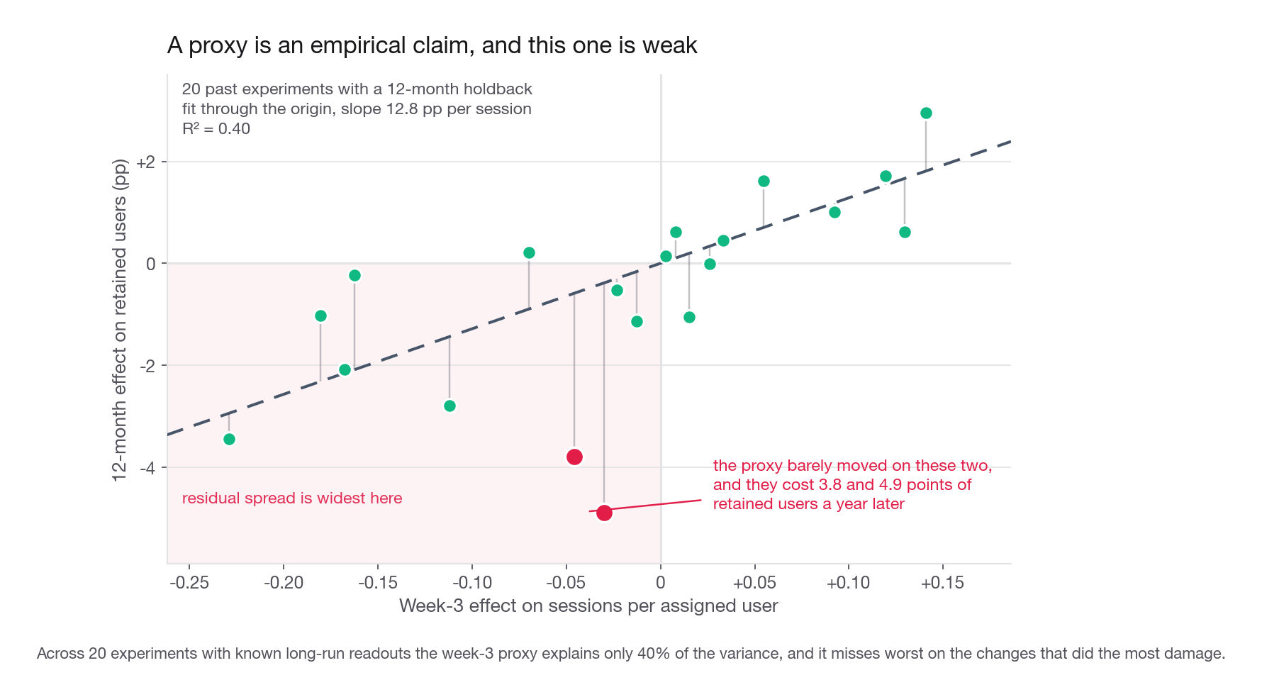
It has been validated on past experiments where you eventually saw the truth. A proxy is an empirical claim about your product, not a definition, so it must be fit and checked against experiments with known long-run readouts.
Condition three is where good teams do the real work: keep a library of every experiment that ran a long holdback, regress the long-run effect on the candidate short-run effect across those experiments, and report the residual spread. A proxy with an R-squared of 0.4 across twenty past experiments is a weak instrument, and you should say so rather than pretend it is a measurement.
Proxy candidates for the two canonical levers
| Lever | Weak proxy candidates | Proxies that carry the mechanism |
|---|---|---|
| Ad load | Revenue per session, click rate | Sessions per assigned user in weeks 3 and 4, session length distribution at the 25th percentile, share of sessions abandoned mid-item |
| Push volume | Push open rate, sessions on send day | Cumulative opt-out rate, system-level permission revocations, mute-this-topic rate, uninstall rate |
| Discounting | Conversion rate, orders per week | Repeat rate of discounted cohorts at day 60, share of second orders that also use a code |
| Click-tuned ranking | Click-through rate | Same-user return rate at day 7, dwell time past the first item, report or hide rate |
Notice the pattern. The good proxies measure whether the user came back, or whether the user actively declined the thing you added, never the interaction you increased. The declines are best because they are cheap to detect and near-impossible to explain away: revoking notification permission is an unambiguous week-one vote about a cost that will not reach revenue for months.
Detecting the creatives that poison the surface
A related question comes up constantly in ad-network interviews: without labels, find the ads that win clicks by degrading the surface they run on. The measurement idea is to look at the same users afterwards, on other inventory.
For each creative, take the users who clicked it, and compare their click rate on everything else in the two weeks before that click to their click rate on everything else in the two weeks after. A creative that delivers what it promises leaves that number unchanged. A creative that misleads leaves the user less willing to trust the whole surface, and their subsequent click rate on unrelated ads drops.
WITH first_click AS (
  SELECT user_id, creative_id, MIN(clicked_at) AS t0
  FROM ad_click
  WHERE clicked_at BETWEEN CURRENT_DATE - 90 AND CURRENT_DATE - 21
  GROUP BY 1, 2
),
windows AS (
  SELECT f.creative_id,
         f.user_id,
         AVG(CASE WHEN i.shown_at BETWEEN f.t0 - 14 AND f.t0 THEN i.was_clicked END) AS ctr_before,
         AVG(CASE WHEN i.shown_at BETWEEN f.t0 AND f.t0 + 14 THEN i.was_clicked END) AS ctr_after
  FROM first_click f
  JOIN ad_impression i
    ON i.user_id = f.user_id
   AND i.creative_id <> f.creative_id
  GROUP BY 1, 2
)
SELECT creative_id,
       COUNT(*) AS clickers,
       AVG(ctr_after - ctr_before) AS trust_delta
FROM windows
WHERE ctr_before IS NOT NULL AND ctr_after IS NOT NULL
GROUP BY 1
HAVING COUNT(*) >= 500
ORDER BY trust_delta ASC
LIMIT 50;
Rank creatives on their own click rate against this trust delta. The ones you want are high on the first and sharply negative on the second: they harvest clicks and leave the surface worse. Once you have that ranked list, treat the extreme tail as labels and train a supervised model on properties available before serving, such as headline text features, landing-page load time, the gap between headline entities and landing-page entities, and advertiser history. That converts a detection problem into a pre-serve blocking problem.
Two caveats to raise first: clickers are not a random sample, so the before-window is essential and matched non-clickers are a useful control; and reversing the sort surfaces creatives that increase subsequent trust, which is a better product idea than blocking.
Holdbacks: the only honest long-run measurement
A proxy is an estimate. A holdback is a measurement. Long-run holdbacks are the mechanism by which a company keeps the ability to know what its own launches did.
Three kinds, and they answer different questions
The global holdback is the one most candidates have never heard of and the one senior interviewers enjoy hearing about. Keep one percent of users on the product as it stood on January first, ship everything to the other 99, read the gap in December. It is the only instrument that catches twelve launches each reading plus 1 percent while the aggregate is negative.
Sizing it
Holdbacks are asymmetric: a small held-out group against a very large treated group. The small arm dominates the variance.
Z_ALPHA, Z_BETA = 1.959964, 0.841621

def holdback_size(p_control, delta_pp, ratio=99.0):
    p1 = p_control
    p2 = p_control - delta_pp / 100.0
    var = p1 * (1 - p1) + p2 * (1 - p2) / ratio
    return int(((Z_ALPHA + Z_BETA) ** 2) * var / (p1 - p2) ** 2) + 1

for d in (3.0, 1.5, 1.0, 0.5, 0.25):
    n = holdback_size(0.70, d)
    print(d, n, round(100 * n / 4_200_000, 3))
3.0 1851 0.044
1.5 7402 0.176
1.0 16653 0.397
0.5 66603 1.586
0.25 266399 6.343At Nightjar's 4.2 million monthly actives and a 70 percent twelve-week retention baseline, a one percent holdback resolves about a 0.6 point retention difference. Carry the scaling law with you: sample size goes as one over the square of the effect, so halving the effect quadruples the holdback. That is the honest sentence to say in an interview: not "we would run a holdback," but "a one percent holdback on our base resolves roughly 0.6 points of retention, and halving the effect quadruples the holdback, so if the effect we care about is 0.3 points we need about four and a half percent held out or we should not claim we measured it."
Flag the approximation before someone else does. The ratio=99 argument pins the allocation at a one percent holdback, so the top three rows are self-consistent and the bottom two understate themselves: at 0.25 points the real split is nearer 1 to 14 than 1 to 99, and the answer is 6.7 percent of the base, not 6.3. Solving for the fraction and its own ratio together gives 0.044, 0.175, 0.394, 1.595, and 6.735 percent. Either way 0.3 points lands near four and a half, 4.41 with the ratio fixed and 4.57 when you let it float.
Operating rules that people get wrong
Never re-randomize. A holdback whose membership refreshes each quarter measures nothing, because the accumulated difference is the entire point.
Hold out the whole surface, not the flag. If held-out users still see the redesigned navigation because it shipped outside the flag, you are measuring a fraction of the change and will conclude it was harmless.
Budget the cost explicitly. One percent held back from a change worth 12 percent revenue costs about 0.12 percent of revenue. Say the number. It is almost always trivially worth it, and saying it out loud is what gets it approved.
Decide the readout date in advance and write it in the launch doc, because the pressure to peek and conclude early is enormous once the launch is already celebrated.
Watch for contamination in social or shared-account products, where held-out users experience the change through people they interact with.
Interview tip: If asked how you would prove a launch from last year actually helped, answer "we would not be able to unless we kept a holdback, so I would start one now for this year's launches" instead of proposing an observational reconstruction that cannot work.
How to argue for a short-term loss
The analysis is the easy half. Getting a team to accept a quarter of worse numbers is the half that decides whether you have influence.
The weak script
"I think we should not ship the ad-load increase. The revenue gain looks real but I am worried about long-term effects on retention, and heavier ad loads have historically been bad for user experience. I would recommend we be cautious here."
Nothing in that is wrong and none of it is decidable. There is no number, no threshold, and no plan, so the meeting resolves in favour of whoever has the revenue target.
The stronger script
"Over thirteen weeks this banked an extra 0.17 USD of contribution per assigned user and raised weekly churn from 3.0 to 5.0 percent. On our standard twelve-month horizon those net to about minus 0.01 USD per user, so this is a wash at best. It breaks even at 1.9 points of extra weekly churn and we measured 2.0, and the interval on that comparison straddles zero, so on our own evidence the two are tied. My recommendation is to not ship at four spots, ship at three and a half by showing the fourth spot only to sessions longer than twelve minutes, which our proxy says captures about 60 percent of the revenue with roughly a third of the churn cost, and put one percent into a twelve-month holdback so that next year we can actually settle this."
That version wins because it uses one currency, gives a break-even the other side can argue with, offers an alternative rather than a veto, and proposes a way to settle the disagreement with evidence later.
Pre-commit, in writing, before the launch
The most valuable habit here has nothing to do with statistics. Before the experiment starts, write down: the horizon, the decision rule at each outcome, the guardrails and their thresholds, and the holdback plan. Circulate it. Get the PM to agree.
This is not process hygiene. Once a result arrives the horizon becomes negotiable, and whoever wants to ship will find a horizon on which shipping is correct. Pre-registering it converts a political argument into an arithmetic one.
Common traps
Reporting per active user instead of per assigned user. If the treatment causes churn, dividing by survivors hides exactly the effect you are hunting, and can even make a harmful change look beneficial because the users it drove away were the low-value ones. Always divide by the assignment denominator.
Treating "retention was not significant" as "retention was unaffected." Two different failures hide behind that sentence and candidates collapse them into one. First, two weeks into a test nobody has a twelve-week retention outcome yet. That endpoint is censored, not underpowered, so no sample size fixes it and there is no minimum detectable effect to quote. Second, on the two-week retention you can observe, 20,000 users per arm resolves about 0.50 points against this dataset's 96.9 percent two-week baseline, or about 1.3 points against a 70 percent twelve-week baseline, while the true week-two gap in the Nightjar panel is 0.17 points. Genuinely below the detectable effect, so invisible by construction, even though the same mechanism reaches 9.9 points by week thirteen. What you must not say is that the test was too small: 40,000 users is roughly fifteen times what a 5 point effect would need. Ask for the follow-up window and then the minimum detectable effect, never just "was it significant."
Extrapolating the observed hazard forever. In the Nightjar data the incremental hazard grows every week because exposure accumulates. Projecting that growth to infinity produces a catastrophic and unbelievable number. Projecting a flat hazard at the week-13 level, as this lesson does, is the defensible middle. Say which assumption you made and show the answer under one alternative.
Comparing revenue on one side to margin on the other. The short-term gain is usually quoted in revenue because that is what the dashboard shows, while the long-term loss lands in contribution. Convert both, or the comparison is meaningless.
Choosing the horizon after seeing the result. The single most common way this analysis gets corrupted, and almost never deliberate. Pre-register it.
Using a proxy that the treatment can bypass. Optimising ad load against "revenue per session" cannot fail: revenue per session is what the change increases. A proxy has to be able to say no.
Refreshing the holdback population. Re-randomizing each quarter destroys the accumulated difference the holdback exists to measure. Membership is permanent for the life of the study.
Assuming every short-term win is a trap. Real free wins exist: faster load times, fixing a broken funnel step, a better search index. If you cannot articulate the mechanism by which a change costs something later, do not invent one. Manufactured skepticism reads as inexperience, not rigour.
Ignoring the competitive clock. A change that destroys value over 24 months can still be correct if the company will not exist in 24 months without the revenue. Name the runway constraint rather than pretending it away.
Quick self-check
Answer these out loud, in full sentences, as if the interviewer just asked them.
A test raised revenue per user 11 percent over two weeks with no significant retention change. What is the first question you ask, and why is "was retention significant" the wrong version of it?
Ad load and push notification volume are both short-term wins with long-term costs. Name the structural difference between them and explain how it changes the experiment you would design.
You have banked contribution from the test window and a forward projection. Walk through how the ship or do-not-ship answer changes across 26, 52, and 104 week horizons, and say who should choose the horizon and when.
What are the three conditions a proxy metric has to satisfy, and which one do candidates usually skip? Give an example of a proxy that passes the first condition and fails the second.
Your product has 4.2 million monthly actives and a 70 percent twelve-week retention rate. You are asked to hold back one percent for a year. What effect size can you resolve, and what does it cost in revenue if the launches ship a combined 8 percent gain?
Give the two-sentence version of the argument for not shipping a change that adds 0.17 USD per user this quarter, phrased so a revenue-targeted PM can disagree with a specific number rather than with your judgment.