1.3 Decision Trees as a Segment Finder
Find the core decision, design, or behavior signal.
Turn the lesson into a concise response blueprint.
Name the trap you would avoid in a real interview.
Use these checkpoints as your reading path before diving into the full lesson.
- 1Why this matters in interviews
- 2The data we are reading
- 3Fitting a tree for carving, not for acc...
- 4Reading the tree top down
- 5What a node actually reports
A growth PM at Cadence wants to know which weekly push notifications are worth sending and which ones are quietly training members to swipe the app away. A coefficient table cannot settle that. It reports how far one lever shifts the odds on average; the PM needs named groups, each with a volume, a rate, and a rule the campaign tool can run on Monday. A shallow decision tree produces that shape by construction. This lesson covers fitting one for carving rather than accuracy, reading it node by node, proving its segments survive new data, and handing over a targetable audience.
Why this matters in interviews
Interviewers reach for a tree the second a prompt says "which members", "segment", or "cutoff". It is the only technique on your menu whose output already is an audience: a coefficient says how much, a leaf says who and how many. Here is the version that gets a candidate filed under junior:
A weak answer: "I would fit a decision tree, pull the feature importances, and report that send hour is the most important variable."
Importance is a unitless scalar nobody can hold. It says nothing about where the boundary falls, how much volume sits on each side, or what changes tomorrow. Now the senior version:
A strong answer: "The tree cuts first at 19:00. Below that line sits 76.8 percent of weekly volume tapping at 3.90 percent; at or above it sits 23.2 percent tapping at 5.70 percent. But that cut only buys 0.000115 of Gini against a root impurity of 0.0826, and a hand-built window of 07 to 08 plus 19 to 21 buys 0.000156, which CART cannot express in a single cut. So I would report the evening window as the leading structure and say plainly that it is not a runaway winner."
The second answer carries two sizes, two rates, the gain, and an honest statement of the winner's margin. That last clause separates a candidate who read a tutorial from one who has shipped one.
Interviewers also probe what a tree cannot do. Candidates treat the diagram as a ranked list of what matters. It is not. Everything below the root is conditional on the questions above it, a cheap and real lever can be absent entirely, and your encoding can suppress a variable that is a clean binary in the business. All three failures show up below.
Interview tip: Never state a tree finding without three numbers attached: the rule, the share of volume it covers, and the outcome rate inside it. A split quoted without a size is trivia, not a recommendation.
The data we are reading
Cadence is a subscription audiobook app with roughly 320,000 active members, each receiving one "Picked for you" push notification per week. One row below is one notification sent, and the label records whether the member opened the app from it inside twenty four hours.
| Column | Type | Meaning |
|---|---|---|
notif_id | integer | Unique per notification sent |
copy_length | brief / detailed | One short line of body text, or a fuller three-line blurb |
greeting | named / generic | Opens with the member's first name, or does not |
send_hour | 6 to 22 | Local hour the scheduler released the push |
weekday | Mon to Sun | Local day of week |
market | US / UK / CA / AU / DE | Member's billing market |
titles_finished | count | Lifetime audiobooks completed before this send |
days_since_last_listen | count | Recency at the moment of sending |
tapped | 0 / 1 | Label: opened the app from this push within 24 hours |
One design fact governs everything below. The scheduler assigns copy_length, greeting, send_hour and weekday from a rotation that ignores who the member is, so those four are effectively randomized; the other three describe who the member already was, so differences there are descriptive only. This block builds a deterministic stand-in, and every figure below comes from running it.
import numpy as np
import pandas as pd

SEED = 20260826
rng = np.random.default_rng(SEED)
N = 80_000

weekdays = np.array(["Mon", "Tue", "Wed", "Thu", "Fri", "Sat", "Sun"])
markets = np.array(["US", "UK", "CA", "AU", "DE"])

copy_length = rng.choice(["brief", "detailed"], N)
greeting = rng.choice(["named", "generic"], N)
send_hour = rng.integers(6, 23, N)
weekday = rng.choice(weekdays, N, p=[.16, .16, .16, .16, .14, .11, .11])
market = rng.choice(markets, N, p=[.46, .18, .14, .12, .10])
titles_finished = rng.poisson(3.1, N)
days_since_last_listen = rng.geometric(0.11, N) - 1

z = np.full(N, -3.85, dtype=float)
z += np.where(copy_length == "brief", 0.34, 0.0)
z += np.where(greeting == "named", 0.22, 0.0)
z += np.where(np.isin(weekday, ["Sat", "Sun"]), -0.47, 0.0)
z += 0.58 * np.exp(-((send_hour - 8.5) ** 2) / 5.5)      # commute peak
z += 0.71 * np.exp(-((send_hour - 20.0) ** 2) / 6.5)     # evening peak
z += np.select([market == "DE", market == "AU"], [-0.93, -0.14], 0.0)
z += 0.31 * np.log1p(titles_finished)
z += -0.028 * np.minimum(days_since_last_listen, 45)
z += 0.86 * ((market == "DE") & (copy_length == "detailed"))          # interaction
z += 0.52 * ((days_since_last_listen > 21) & (greeting == "named"))   # interaction

notifs = pd.DataFrame({
    "notif_id": np.arange(1, N + 1),
    "copy_length": copy_length,
    "greeting": greeting,
    "send_hour": send_hour,
    "weekday": weekday,
    "market": market,
    "titles_finished": titles_finished,
    "days_since_last_listen": days_since_last_listen,
    "tapped": rng.binomial(1, 1.0 / (1.0 + np.exp(-z))),
})
Eighty thousand notifications, 3,452 taps, a base rate of 4.315 percent. Every leaf gets compared against that number and nothing else.
Fitting a tree for carving, not for accuracy
Tuned for accuracy, a tree grows until each leaf is nearly pure and you finish with two hundred leaves nobody can act on. Tuned for reading, it stays printable, every leaf big enough to campaign against.
from sklearn.tree import DecisionTreeClassifier, export_text

X = pd.get_dummies(notifs.drop(columns=["notif_id", "tapped"]), drop_first=False)
y = notifs["tapped"]

tree = DecisionTreeClassifier(
    max_depth=4,               # four questions deep, so a leaf reads as one sentence
    min_samples_leaf=1000,     # no leaf smaller than a campaign cell worth building
    min_impurity_decrease=0.00002,  # refuse splits that buy almost nothing
    random_state=0,
).fit(X, y)

print(export_text(tree, feature_names=list(X.columns), show_weights=True))
Four choices, each of which you should be ready to defend.
max_depth=4 is a communication constraint, not a statistical one. A leaf at depth four is a sentence with four clauses; at depth seven it is a paragraph nobody translates into a campaign builder.
min_samples_leaf=1000 comes from Cadence operations, not the data. A thousand weekly sends is the smallest cell their tooling schedules separately, so a two hundred row leaf is not a segment however tidy it looks.
min_impurity_decrease is the knob everyone leaves at zero and then wonders why the bottom of the tree is static. Here it matters more than usual: the knob is not scale free. Root Gini is 2 * 0.04315 * 0.95685 = 0.0826, so every candidate split buys a number in the fourth or fifth decimal place. The 0.0005 quoted in tutorials refuses every split and hands you a bare stump, though on a 20 percent base rate it is sensible. Set it as a fraction of root impurity and check what it prunes.
drop_first=False is deliberate. Dropping a reference level suits a regression, where the omitted category folds into the intercept. A tree has no intercept, so dropping a level only removes a candidate question and can silently change the winner.
Here is what came back.
|--- send_hour <= 18.50
|   |--- copy_length_detailed <= 0.50
|   |   |--- market_DE <= 0.50
|   |   |   |--- send_hour <= 10.50
|   |   |   |   |--- weights: [9908.00, 612.00] class: 0
|   |   |   |--- send_hour >  10.50
|   |   |   |   |--- weights: [16276.00, 718.00] class: 0
|   |   |--- market_DE >  0.50
|   |   |   |--- weights: [3036.00, 61.00] class: 0
|   |--- copy_length_detailed >  0.50
|   |   |--- days_since_last_listen <= 7.50
|   |   |   |--- weights: [17869.00, 684.00] class: 0
|   |   |--- days_since_last_listen >  7.50
|   |   |   |--- weights: [11980.00, 321.00] class: 0
|--- send_hour >  18.50
|   |--- days_since_last_listen <= 10.50
|   |   |--- copy_length_detailed <= 0.50
|   |   |   |--- weights: [6315.00, 482.00] class: 0
|   |   |--- copy_length_detailed >  0.50
|   |   |   |--- weights: [6296.00, 360.00] class: 0
|   |--- days_since_last_listen >  10.50
|   |   |--- weights: [4868.00, 214.00] class: 0
Eight leaves, four variables in play, and three of the seven predictors never asked about at all. Hold that last observation.
Reading the tree top down
What a node actually reports
Every node carries four things and candidates routinely misread two. The question is a threshold sitting halfway between two observed values, which is why the printout says 18.50 rather than 19; read it aloud as "released at 19:00 or later", and read market_DE <= 0.50 as "not Germany". The row counts give segment size, what a PM wants right after the rate. The class proportion is the segment's tap rate: compare it to the root rate of 4.315 percent, never to 0.5. The impurity score, Gini by default, is 2p(1-p), peaking at 0.5 on a fair coin and falling to zero on a pure node. It is bookkeeping for choosing splits, not a number you hand a product team.
Two reading errors deserve names. The predicted class label is worthless here: at a 4.3 percent base rate every node is class 0, including the best leaf at 7.09 percent, so read the rate instead. And under class_weight="balanced" the numbers in value are reweighted pseudo-counts, so recompute rates from the raw frame.
The first split is the headline, and its margin matters more
Work the root arithmetic by hand once so you can defend it under pressure. The root tap rate is 0.04315, so Gini is 2 * 0.04315 * 0.95685 = 0.082576. The left child holds 61,465 notifications, 76.83 percent of volume, tapping at 3.898 percent, Gini 0.074924; the right child holds 18,535 tapping at 5.697 percent, Gini 0.107455. Weighted child impurity is 0.7683 * 0.074924 + 0.2317 * 0.107455 = 0.082461, so the split bought 0.000115.
That number alone means nothing. What decides whether you lead with the root is its distance to the runners-up, measurable without the fitted object.
def gini(p):
    return 2 * p * (1 - p)

root = gini(notifs["tapped"].mean())

def impurity_drop(mask):
    w = mask.mean()
    a = notifs.loc[mask, "tapped"].mean()
    b = notifs.loc[~mask, "tapped"].mean()
    return root - (w * gini(a) + (1 - w) * gini(b))

candidates = {
    "send_hour in 7,8,19,20,21": notifs["send_hour"].isin([7, 8, 19, 20, 21]),
    "send_hour 12 to 17": notifs["send_hour"].between(12, 17),
    "send_hour <= 18": notifs["send_hour"] <= 18,
    "copy_length is brief": notifs["copy_length"].eq("brief"),
    "weekday is Sat or Sun": notifs["weekday"].isin(["Sat", "Sun"]),
    "days_since_last_listen <= 10": notifs["days_since_last_listen"] <= 10,
    "market is DE": notifs["market"].eq("DE"),
}
for label, mask in candidates.items():
print(f"{label:28s} {mask.mean():.3f} {impurity_drop(mask):.6f}")| Candidate first split | Share left | Rates, left vs right | Impurity bought |
|---|---|---|---|
send_hour in 07, 08, 19, 20, 21 | 0.292 | 5.69% vs 3.75% | 0.000156 |
send_hour between 12 and 17 | 0.356 | 3.26% vs 4.90% | 0.000122 |
send_hour <= 18 | 0.768 | 3.90% vs 5.70% | 0.000115 |
copy_length is brief | 0.499 | 4.99% vs 3.64% | 0.000091 |
weekday is Sat or Sun | 0.221 | 3.06% vs 4.67% | 0.000089 |
days_since_last_listen <= 10 | 0.723 | 4.70% vs 3.31% | 0.000077 |
market is DE | 0.101 | 2.89% vs 4.48% | 0.000046 |
Three things to say about this table, and a candidate who says all three is done arguing.
First, the winner does not run away with it. The chosen root beats the best non-timing candidate by a factor of 1.26. Where a top split buys six times the runner-up you may call it dominant structure; here you may not, and pretending otherwise gets you embarrassed at the next refit.
Second, the top row is a split the tree could not have made. A window of the two commute hours plus the three evening hours buys 0.000156, thirty six percent more than the cut CART chose. CART asks only one-sided questions on an ordered variable, so it cannot say "07 to 08 or 19 to 21" in one node and approximates the shape with several cuts instead. Watch it happen: the left branch immediately re-splits on send_hour <= 10.5 to claw back the commute peak it lost at 19:00. A numeric column asked about twice on one path is non-monotone, and a single threshold is the wrong summary of it.
Third, weekday is Sat or Sun buys 0.000089, essentially tied with copy_length, yet no weekday column appears in the fitted tree. That is an encoding artifact, and it gets its own section.
Interview tip: When you present a root split, quote the impurity it bought next to the impurity the runner-up would have bought. "It wins, but only by a quarter" is far more credible than naming a winner and stopping.
Walking down one branch
Among the 61,465 sends released before 19:00 the tree asks about copy length. Inside brief copy it pulls out Germany: German brief sends tap at 1.97 percent against 4.83 percent elsewhere. It then chops the non-German brief sends at 10:30, separating a morning block at 5.82 percent from the midday stretch at 4.23 percent. Detailed copy before 19:00 never gets a market question; it splits on recency instead, 3.69 percent within the week against 2.61 percent for those away longer.
Notice what happened. The tree asked about Germany inside the brief branch and declined inside the detailed branch. That asymmetry is the model saying the German penalty exists for one copy variant only, the most valuable fact in this dataset.
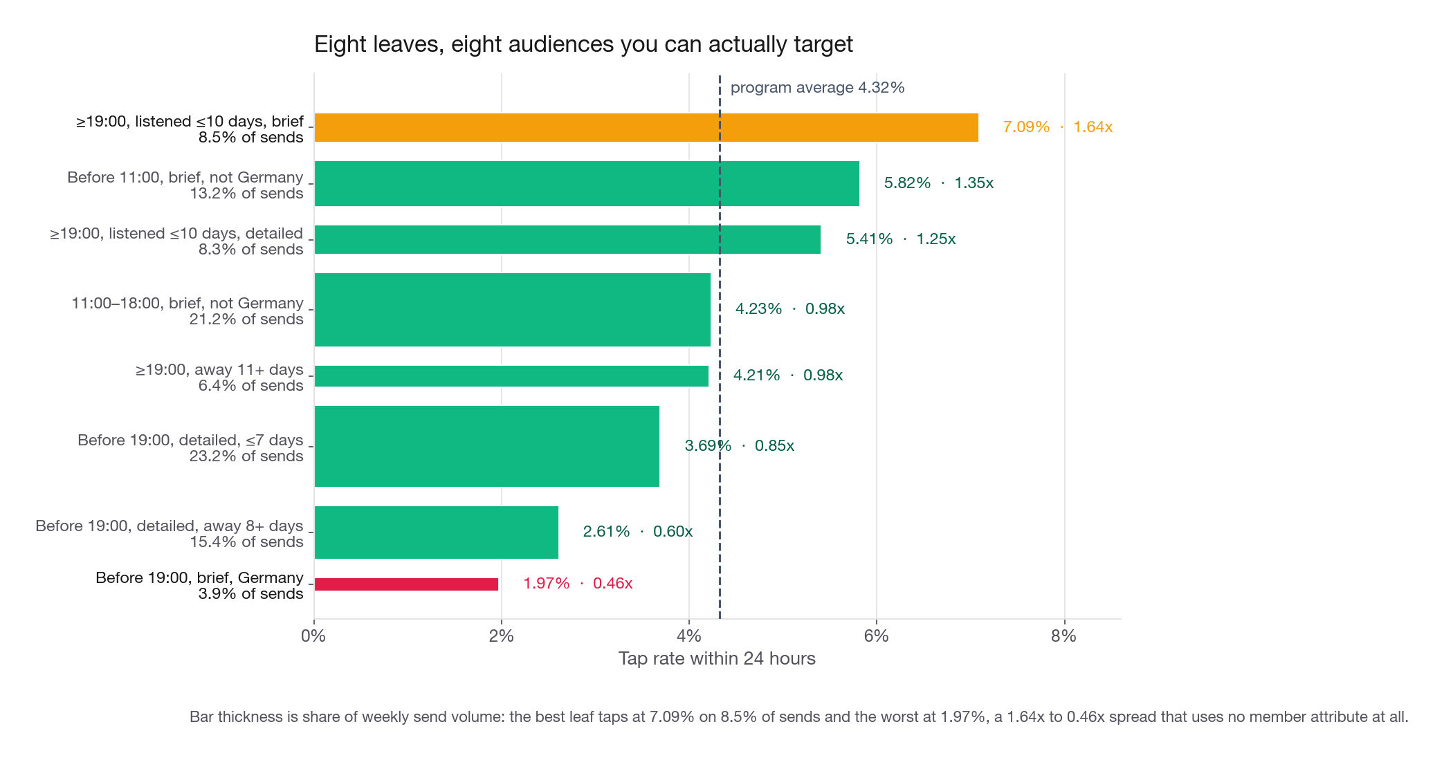
The evening branch is shorter. Sends at 19:00 or later split on recency at ten and a half days, then, for the recent group, on copy length: brief taps at 7.09 percent, detailed at 5.41 percent. Read the best leaf aloud: "A brief push after 19:00 to a member who listened within ten days. Eight and a half percent of weekly volume at 7.09 percent, 1.64 times the program average." That is the deliverable.
The leaf table is what you hand over
Do not hand over the diagram. Hand over the leaves as a table sorted by lift.
report = (
    notifs.assign(leaf=tree.apply(X))
          .groupby("leaf")
          .agg(sends=("tapped", "size"), taps=("tapped", "sum"))
)
report["tap_rate"] = report["taps"] / report["sends"]
report["share"] = report["sends"] / len(notifs)
report["lift"] = report["tap_rate"] / notifs["tapped"].mean()
print(report.sort_values("lift", ascending=False).round(4))| Leaf rule | Sends | Share | Tap rate | Lift |
|---|---|---|---|---|
| 19:00 or later, listened within 10 days, brief | 6,797 | 8.5% | 7.09% | 1.64x |
| Before 11:00, brief, not Germany | 10,520 | 13.2% | 5.82% | 1.35x |
| 19:00 or later, listened within 10 days, detailed | 6,656 | 8.3% | 5.41% | 1.25x |
| 11:00 to 18:00, brief, not Germany | 16,994 | 21.2% | 4.23% | 0.98x |
| 19:00 or later, away 11 days or more | 5,082 | 6.4% | 4.21% | 0.98x |
| Before 19:00, detailed, listened within 7 days | 18,553 | 23.2% | 3.69% | 0.85x |
| Before 19:00, detailed, away 8 days or more | 12,301 | 15.4% | 2.61% | 0.60x |
| Before 19:00, brief, Germany | 3,097 | 3.9% | 1.97% | 0.46x |
Eight rows summing to the whole population, each a rule someone can paste into a targeting tool. That mutually exclusive, collectively exhaustive coverage is what a coefficient table never gives you: a regression hands you an odds ratio on the evening window, not a partition where every notification lands in one bucket of known size, ordered by worth. The spread runs 1.64x to 0.46x, and none of it touches who the members are.
Everything below the root is conditional
The root is a claim about the whole population. Every split beneath it is a claim about a subgroup defined by the questions above. When the tree cuts on market_DE inside the "before 19:00, brief copy" branch it is silent about Germany anywhere else: nothing on the German penalty for detailed copy, nothing in the evening, nothing overall.
That bites the moment someone asks what happens if we move every eligible send into the evening. The tree cannot answer it. It answers a narrower question: among recent listeners on brief copy, an evening release taps at 7.09 percent against 4.37 percent for the same copy to the same people between 11:00 and 18:00. The population-wide answer needs a marginal effect averaged over everyone, or a live experiment. Trees understate broad levers, because something that helps everybody a little never wins an argmax against a variable that cleaves the population. Pair the tree with a second technique, or you will undervalue every uniform improvement your team could ship.
Interview tip: If an interviewer asks for the overall effect of shifting the whole program to evening sends, say out loud that the tree cannot support that number and name what would: an averaged marginal effect over the full population, or a randomized holdback.
Interactions: the structure the tree surfaced unprompted
A main-effects logistic regression fits one coefficient for German market and one for detailed copy, and predicts that German members on detailed copy are the worst cell in the program. It is wrong, and a regression can be made to admit it: type a Germany-by-brief product term into the model and the truth falls out, which is what the previous lesson did. But you have to suspect the term before you can type it. The tree needed no prompt: it asked about Germany inside the brief branch and declined inside the detailed one, and that asymmetry is the interaction.
grid = (
    notifs.assign(bloc=np.where(notifs["market"].eq("DE"), "DE", "rest"))
          .groupby(["bloc", "copy_length"])["tapped"]
          .agg(["mean", "size"])
)
print(grid.round(4))| Segment | Brief copy | Detailed copy | Gap, brief minus detailed |
|---|---|---|---|
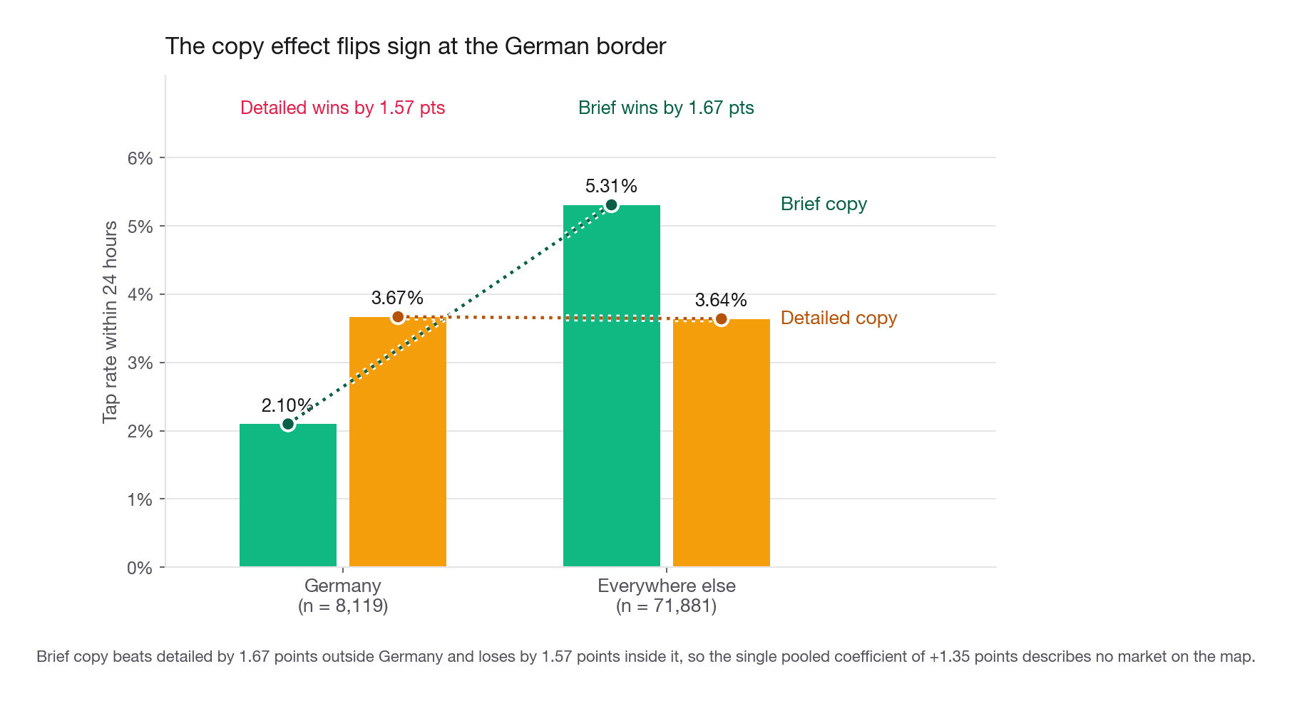
| Germany | 2.10% (n = 4,001) | 3.67% (n = 4,118) | -1.57 pts |
| Everywhere else | 5.31% (n = 35,936) | 3.64% (n = 35,945) | +1.67 pts |
| All markets | 4.99% (n = 39,937) | 3.64% (n = 40,063) | +1.35 pts |
The sign flips. Outside Germany brief beats detailed by 1.67 points; inside Germany detailed beats brief by 1.57, and German detailed sends land at 3.67 percent, indistinguishable from the 3.64 percent detailed rate elsewhere. Germany is not a weak notification market. It is a market where the short blurb fails and the fuller one performs normally.
A single "brief copy" coefficient averages a positive and a negative into +1.35 points, a number describing no market on the map. Act on it and you push the short variant globally, hand German members the one variant that fails them, and spend a quarter arguing about whether Germany has a translation problem.
Because the scheduler assigns copy_length, greeting and send_hour from a rotation that ignores the member, the copy contrast above is close to randomized and you can talk about it causally. Recency and market are not: someone away a month differs from a daily listener in a hundred unobserved ways. Say which splits are assigned and which are self-selected. Most candidates never draw that line, and it is the difference between a recommendation and a correlation.
Interview tip: When you report an interaction, give the number for each side separately and never the average. "Detailed wins by 1.6 points in Germany and loses by 1.7 everywhere else" is actionable; "detailed is 1.4 points worse overall" describes nobody.
Depth and complexity: two jobs, two settings
Depth trades predictive accuracy against usable segments, and the trade turns over faster than people expect.
from sklearn.model_selection import train_test_split
from sklearn.metrics import roc_auc_score

tr, te = train_test_split(np.arange(len(y)), test_size=0.3,
                          random_state=5, stratify=y)
for depth in [1, 2, 3, 4, 6, 10, None]:
    fit = DecisionTreeClassifier(max_depth=depth, min_samples_leaf=200,
                                 random_state=0).fit(X.iloc[tr], y.iloc[tr])
    sizes = pd.Series(fit.apply(X.iloc[tr])).value_counts() / len(tr)
    auc = roc_auc_score(y.iloc[te], fit.predict_proba(X.iloc[te])[:, 1])
    print(depth, fit.get_n_leaves(), int((sizes >= 0.02).sum()), round(auc, 4))
max_depth | Leaves | Leaves holding 2%+ of rows | Train AUC | Holdout AUC |
|---|---|---|---|---|
| 1 | 2 | 2 | 0.5390 | 0.5384 |
| 3 | 8 | 6 | 0.5842 | 0.5580 |
| 4 | 16 | 10 | 0.5995 | 0.5670 |
| 6 | 45 | 13 | 0.6267 | 0.5753 |
| 10 | 144 | 6 | 0.6667 | 0.5822 |
| unlimited | 201 | 0 | 0.6800 | 0.5776 |
Read the last column first and say something uncomfortable out loud. Holdout AUC never clears 0.582 at any depth. This tree is not a predictor: nobody should rank a send queue with it. It describes where the outcome varies, which is legitimate and useful, but say so before someone deploys it.
Now the third column. Depth six gives thirteen leaves holding at least two percent of rows, the most of any setting. Depth ten gives better holdout AUC and six usable leaves. Unlimited depth gives the best training score, a worse holdout score than depth ten, and not one campaignable leaf. Past depth six the two objectives diverge. So: for prediction, tune depth against a holdout metric; for insight, fix depth at three or four, set leaf size from the operational floor, and treat accuracy as a sanity check. At 0.50 the segments are noise; at 0.567 you have real but modest structure.
Instability, and the three checks that make a split credible
Trees are the least stable model you will put in front of an executive. Perturb a few percent of rows and the structure rearranges, because each split is an argmax over many nearly tied candidates. Show a PM one diagram in March and a different one in April and you have spent credibility you do not get back.
Check one: bootstrap the split
Resample rows with replacement, refit a stump, count how often the same variable and threshold win.
boot = np.random.default_rng(7)
picks = []
for _ in range(60):
    rows = boot.integers(0, len(y), len(y))
    stump = DecisionTreeClassifier(max_depth=1, min_samples_leaf=1000,
                                   random_state=0).fit(X.iloc[rows], y.iloc[rows])
    j = stump.tree_.feature[0]
    picks.append(f"{X.columns[j]} <= {stump.tree_.threshold[0]:.1f}")
print(pd.Series(picks).value_counts())
send_hour <= 18.5 41
copy_length_brief <= 0.5 10
send_hour <= 17.5 5
copy_length_detailed <= 0.5 1
days_since_last_listen <= 10.5 1
days_since_last_listen <= 12.5 1
days_since_last_listen <= 8.5 1Resampling all eighty thousand rows, the send-hour family wins the root in 46 of 60 draws and copy length takes it in 11; the exact threshold 18.5 survives only 41 times. The honest sentence is "timing wins the root about three quarters of the time and copy length is a live alternative", not "the tree splits on send hour".
Shrink the resample to four thousand rows, roughly one mid-sized market in a week, and the root becomes a scramble: send hour 14, copy length 13, recency 12, four further variables sharing the remaining 21. Sample size does most of the work behind any stability you observe, so quote it beside the claim. A root that holds on 80,000 rows may be a coin flip on the slice a regional team has.
Check two: hold rows out before you fit, not after
The tree searched thousands of candidate splits, so its winning leaves were selected on the rows that produced their rates. Correcting that needs the right order: withhold rows first, then let the search run on the rest.
train_rows, hold_rows = train_test_split(
    notifs, test_size=0.35, random_state=11, stratify=notifs["tapped"])

honest = DecisionTreeClassifier(max_depth=4, min_samples_leaf=1000,
                                min_impurity_decrease=0.00002,
                                random_state=0).fit(X.loc[train_rows.index],
                                                    y.loc[train_rows.index])
print(export_text(honest, feature_names=list(X.columns), show_weights=True))
The uncomfortable result comes first: the evening branch does not survive. Fitted on 65 percent of the rows at the same depth and leaf floor, the tree asks titles_finished <= 4.5, then weekday_Mon, then greeting_generic, where the full-data tree asked recency and then copy length. The daytime branch is steadier, copy then Germany then hour, with the morning cut drifting from 11:00 to 12:00. The branch that produced the most quotable sentence is the branch that moved.
Now the shrink. Freeze that tree's own best leaf as text and score it on the untouched 35 percent.
base = notifs["tapped"].mean()

def honest_winner(df):
    return (df["send_hour"] >= 19) & (df["titles_finished"] >= 5)

for name, frame in [("train", train_rows), ("holdout", hold_rows)]:
    seg = honest_winner(frame)
    rate = frame.loc[seg, "tapped"].mean()
    print(name, int(seg.sum()), round(seg.mean(), 4), round(rate, 4),
          round(rate / base, 2))
train 2371 0.0456 0.0751 1.74
holdout 1359 0.0485 0.0699 1.62An evening send to a member with five or more finished titles taps at 7.51 percent on the rows it was chosen from and 6.99 percent on the rows it was not, lift 1.74 down to 1.62. That half point is the winner's curse, and it is the pass condition: an argmax over thousands of comparisons should come back slightly weaker on untouched rows. A leaf that arrives at 3x lift and holds at 1.2x was an artifact; drop it quietly.
The version that circulates splits in the wrong order, and its arithmetic is worth seeing once so you never run it. Freeze the headline leaf, then partition the same 80,000 rows the tree was already fitted on. Train: 291 taps over 4,377 rows, 6.65 percent. Holdout: 191 over 2,420, 7.89 percent. Add them: 482 over 6,797, the 7.09 percent leaf exactly. The halves partition one in-sample number, so whichever lands under 7.09 forces the other over it, and the 7.89 is the complement of the 6.65 rather than evidence. The German leaf does the same, 36 of 1,976 and 25 of 1,121 summing to the 61 of 3,097 you started with. Selection bias cannot be measured against rows that were part of the selection. Read the leaf table as in-sample maxima: the honest refit does not even re-select the 7.09 percent leaf, so quote it with that caveat and ship against the lower end of the range.
Check three: mask the split variable and see what fills the hole
Almost nobody runs this check, and it is the one that prevents an embarrassing recommendation. Does the root variable carry its own information, or stand in for something that tells a different story?
cols = X.columns.drop("send_hour")
masked = DecisionTreeClassifier(max_depth=4, min_samples_leaf=1000,
                                min_impurity_decrease=0.00002,
                                random_state=0).fit(X[cols], y)
print(pd.Series(masked.feature_importances_, index=cols).nlargest(4).round(3))
print((notifs["send_hour"] <= 18).eq(notifs["copy_length"].eq("detailed")).mean())
Drop send_hour and copy length takes the root, with Germany, recency and Sunday filling the rest. Crucially the new partition agrees with the old one on 50.2 percent of rows, exactly chance. Nothing here is a shadow of send hour, so the timing finding is safe to build a roadmap on. Had agreement come back at 90 percent you would have two columns encoding one fact, and your story would turn on which won an argmax by a hair. High agreement means stop and work out which variable is upstream.
What the tree did not tell you
The most instructive result in this fit is a variable that never appears. weekday is absent from the depth-four tree and every weekday dummy has an importance of exactly zero. A candidate reporting only tree output would tell the PM that day of week does not matter. It matters a great deal.
| Segment | Weekend sends | Weekday sends | Gap |
|---|---|---|---|
| All notifications | 3.06% (n = 17,684) | 4.67% (n = 62,316) | -1.61 pts |
| Released 19:00 or later | 3.95% (n = 4,023) | 6.18% (n = 14,512) | -2.23 pts |
| Released before 19:00 | 2.80% (n = 13,661) | 4.21% (n = 47,804) | -1.42 pts |
Weekend sends tap at roughly two thirds the weekday rate, and that ratio holds all day: 0.66 before 19:00, 0.64 inside the evening window, 0.655 overall. Read the Gap column instead and you will invent an interaction that is not there. Fit tapped ~ evening + weekend + evening:weekend as a logit and the interaction term comes back at -0.046 with a p-value of 0.66, a flat null. Do the arithmetic by hand once: apply a constant odds multiplier of 0.63 to the 6.18 percent weekday evening rate and you land on 3.95 percent, the weekend evening rate to the decimal, and the -2.23 point gap drops out of the link with no interaction in the data at all. The gap is wider in the evening because the base rate there is higher. Run the same term on the percentage-point scale and it returns -0.81 points at p = 0.049, apparently a finding, of which about five sixths is the link. Weekend is a main effect: the evening lift is 1.47x on weekdays against 1.41x on weekends.
Two mechanisms produce that silence and telling them apart is the skill. First, budget: depth four is four questions, and timing, copy and market consume them all. Second, encoding, the real culprit here. As a grouped indicator, weekend versus weekday buys 0.000089, tied with copy length at 0.000091 and ahead of every recency or market cut in the candidate table. One-hot forces the tree to ask about one day at a time, and the best single-day question, Sunday against the rest, buys only 0.000061. The tree never gets to ask the question that would have won, because the encoding does not contain it.
G = X.drop(columns=[c for c in X.columns if c.startswith("weekday_")]).copy()
G["is_weekend"] = notifs["weekday"].isin(["Sat", "Sun"]).astype(int)
grouped = DecisionTreeClassifier(max_depth=3, min_samples_leaf=1000,
                                 min_impurity_decrease=0.00002,
                                 random_state=0).fit(G, y)
print(export_text(grouped, feature_names=list(G.columns), show_weights=True))
At depth three the grouped tree splits the evening branch on is_weekend immediately, which the one-hot tree fails to do at any depth up to five. Push it to depth four and its best leaf, a brief evening push on a weekday to a recent listener, reaches 7.71 percent on 5,318 sends against 7.09 percent for the one-hot best leaf. Better encoding, better carve, same depth and leaf floor.
Watch what that tree does not do, though. It leaves the daytime branch alone, which reads as confirmation that the weekend penalty lives in the evening. It is not. A constant odds ratio buys the most Gini where the base rate is highest, so a pure main effect surfaces in the strongest branch first and nowhere else. That asymmetry is the splitting criterion talking, not the data.
The general lesson: absence from a shallow tree is evidence of nothing. Before calling a lever dead, cross-tabulate it inside the largest leaves, group its levels the way the business does, and refit.
Greeting is this section's second casualty, and a cleaner one, because no encoding is at fault. It buys little among active members and a great deal among lapsed ones.
lapsed = notifs["days_since_last_listen"] > 21
print(notifs.groupby([lapsed, "greeting"])["tapped"].agg(["mean", "size"]).round(4))| Segment | Named greeting | Generic greeting | Gap | Ratio |
|---|---|---|---|---|
| Away 22 days or more | 4.22% (n = 2,985) | 2.15% (n = 3,165) | +2.07 pts | 1.96x |
| Away 21 days or fewer | 4.88% (n = 37,069) | 3.94% (n = 36,781) | +0.95 pts | 1.24x |
Among members away more than three weeks, using their first name nearly doubles the tap rate; among everyone else it buys under a point. That ships in an afternoon for one merge field, aimed exactly at the population a winback program exists to reach. The depth-four tree misses it because the lapsed group is 7.7 percent of volume and could not out-compete timing and copy for the four questions allowed. Set min_impurity_decrease to zero at the same depth and greeting appears in two nodes. Weekday lost to the encoding, greeting lost to the budget, and the diagram has nothing to say about either.
From a leaf to a targetable audience
A finding is not shipped until it is a query and a number.
Cadence pushes about 320,000 notifications a week, so a quarter is roughly 4.16 million sends carrying about 179,500 taps. The midday trough, hours 12 through 17, absorbs 35.6 percent of that volume, roughly 1.48 million sends tapping at 3.26 percent. The evening block, hours 19 through 21, taps at 5.97 percent. Because the scheduler assigns the hour independently of the member, that 2.71 point gap is a credible causal contrast, not a selection effect.
Relocating every trough send into the evening block is worth about 40,100 additional opens per quarter. Operations can move a little over half that volume once quiet hours, time zones and evening capacity are respected, so call it 22,000 opens, 12.3 percent more taps than the program produces today. At 0.28 USD per incremental opened session that is roughly 6,200 USD a quarter from a scheduler change. The copy rule is larger and cheaper: brief copy everywhere except Germany, detailed in Germany, is worth about 34,600 extra opens a quarter, a 19.3 percent gain, for one conditional in the template selector. Present that first.
The rule itself becomes a query:
SELECT m.member_id,
       m.market,
       m.days_since_last_listen
FROM   members            AS m
JOIN   push_preferences   AS p USING (member_id)
WHERE  m.days_since_last_listen <= 10
  AND  m.market <> 'DE'
  AND  p.push_opt_in IS TRUE
  AND  p.quiet_hours_start >= TIME '21:30'
  AND  p.weekly_push_count < p.frequency_cap
Note the last three conditions, which the tree knows nothing about. Reachable audience is always smaller than leaf size, and quoting a leaf count as an audience count loses a PM's trust the moment the campaign ships at half the promised volume.
The evening threshold also has a second life as scheduling policy rather than a campaign. Nineteen hundred hours is defensible because it was optimized against a behaviour Cadence cares about instead of chosen by feel. One caveat: the tree cut where the hour best separates tapping, and tapping is not listening. If the policy will govern a roadmap, refit the stump against minutes listened the following week and see whether the knee moves. Sometimes it lands two hours earlier, and that decides which shift operations staffs for a year.
Common traps
Reporting feature importance instead of splits. Gini importance is unitless, unstable, and biased toward high-cardinality variables. The fix: report the split, both sizes and both rates; rank variables with permutation importance on holdout rows.
Leaving min_impurity_decrease at a value you read somewhere. Here root Gini is 0.0826 and 0.0005 prunes the tree to a bare stump. The fix: compute root impurity first, set the floor as a fraction of it, and print the leaf count.
Reading a deep split as a global statement. The German split sits inside the brief-copy daytime branch and says nothing about Germany elsewhere. The fix: prefix every finding with its conditioning path, and use an averaged marginal effect for population-wide numbers.
Concluding a variable does not matter because the tree skipped it. Weekday is worth 1.61 points and appears nowhere. The fix: cross-tabulate it inside the largest leaves, group its levels the way the business does, refit.
Letting one-hot encoding hide a grouped effect. Weekend as a single flag ties with copy length; the best single day loses to it. The fix: when a categorical's levels clearly cluster, build the grouped indicator by hand and let the tree choose.
Promising leaf size as audience size. Opt-in status, quiet hours, suppression lists and frequency caps all shrink the reachable slice. The fix: run the rule against production tables with the operational filters attached first.
Reading a bigger point gap as an interaction. The weekend penalty is 2.23 points in the evening and 1.42 before it, yet the interaction is null, -0.046 at p = 0.66. Identical odds offsets make bigger point gaps wherever the base rate is higher. The fix: test on the scale the model fits, and quote the ratio next to the points.
Validating a leaf on rows the tree was fitted on. Splitting the fitting data afterwards only partitions one in-sample number. The fix: hold rows out before anything is fitted.
Confusing an assigned split with a self-selected one. Hour and copy are close to randomized; recency and market are not. The fix: label every split as assigned or self-selected, and never propose an intervention on a self-selected split without a test.
Quick self-check
Answer these out loud, in full sentences, as if an interviewer just asked them.
The root split sends 76.8 percent of volume left at 3.90 percent and 23.2 percent right at 5.70 percent. Reconstruct the impurity decrease, then explain why you would still refuse to call it the dominant structure in the data.
A window of hours 07, 08, 19, 20 and 21 buys 36 percent more impurity than the split the tree chose. Explain the property of CART that prevents that split, and name the symptom in the fitted tree that gives it away.
Germany taps at 2.10 percent on brief copy and 3.67 percent on detailed, while every other market runs 5.31 and 3.64 percent. State what a main-effects model predicts for German detailed sends, why it is wrong, and what the tree did that gave it away.
Every weekday dummy has an importance of zero, yet weekend sends tap 1.61 points below weekday sends. Give the two mechanisms behind that silence, say which dominates, and the one-line change that fixes it.
Holdout AUC never exceeds 0.582 at any depth, while the leaf table spans 1.97 to 7.09 percent. Reconcile those facts and state what you would and would not let this model be used for.
Refit on 65 percent of the rows and the tree rebuilds the whole evening branch out of different variables, while its best leaf falls from 7.51 percent in training to 6.99 percent on the untouched 35 percent. Explain why that fall is the pass condition rather than the failure, and what you would still claim about the leaf table's 7.09 percent top row.