3.2 Unbalanced Classes: Cut-Offs and Class Weights
Find the core decision, design, or behavior signal.
Turn the lesson into a concise response blueprint.
Name the trap you would avoid in a real interview.
Use these checkpoints as your reading path before diving into the full lesson.
- 1Why this matters in interviews
- 2The setting: Larkfield's booking modal
- 3The trivial classifier, and why accurac...
- 4Two separate questions: is the ranking...
- 5ROC: what it measures and what it conceals
Somebody hands you a classifier that is right 98.3 percent of the time and asks whether it is ready to ship. This lesson is about how to answer that in one sentence, and then about the two levers that actually turn a rare-event model into something a product team can run: moving the decision threshold using costs you can write on a napkin, and reweighting the classes so the model has a reason to look for the rare thing at all. By the end you should be able to derive the correct cut-off from four numbers, say exactly what reweighting changes and what it leaves alone, and spot the moment an interviewer is baiting you into optimizing the wrong quantity.
Why this matters in interviews
Rare outcomes are the outcomes product teams care about. Trial-to-paid conversion runs between half a percent and three percent for most self-serve software, lifecycle click rates land in the same band, and chargebacks, account takeovers and support escalations are all well under one in fifty. Almost every classification question in a product loop is secretly a rare-event question, and the interviewer is watching for one specific failure. It sounds like this:
"I trained a random forest and got 98 percent accuracy on the holdout, so the model is working well."
That answer is close to evidence that you never opened the confusion matrix. When one class is 1.7 percent of the data, emitting the majority label for every row scores 98.3 percent. Accuracy on a heavily skewed label carries almost no information about the thing you were hired to find.
The version that lands:
"With a base rate that low I would not report accuracy at all. I would separate two questions. First, does the score rank users better than chance, which I would read off the precision-recall curve and compare against the base rate as the floor. Second, where do I cut that ranking, which is not a statistics question, it is an expected-value question. Give me the value of catching a positive and the cost of a false alarm and I will hand you the threshold. If the model cannot separate the classes at all and every predicted probability collapses to the base rate, then no threshold helps and I move to class weights so the fit has an incentive to split."
That answer refuses the metric, splits the problem into a ranking part and a decision part, and names the condition under which the first fix fails and the second becomes necessary. That split is the whole lesson.
Interview tip: The instant you hear a base rate under about five percent, say out loud that accuracy is not a metric you will use, and say why in one clause. Interviewers score that sentence heavily and it takes four seconds.
The setting: Larkfield's booking modal
Every number in this lesson comes from one table, so it is worth ten lines of context.
Larkfield is a business workflow-automation product with a self-serve free trial. During onboarding, a subset of trials see an in-app modal offering a fifteen-minute setup call with an implementation specialist. Those calls close at roughly 22 percent, and a closed account is worth about 440 in first-year gross margin, so a booked call carries about 96 in expected margin. The modal is a takeover: it interrupts the onboarding flow, and an internal holdout showed that trials who dismiss it lose about 0.4 percentage points of day-seven activation, worth about 3.20 in expected margin per dismissal.
For eight weeks the growth team showed the modal to everybody, which gives us a clean label. One row is one first-day trial session. The label is whether that session ended in a booked call.
| Column | Type | Meaning |
|---|---|---|
session_id | integer | One row per first-day trial session |
acq_channel | organic / paid_search / partner / webinar / direct | How the trial arrived |
email_domain | corporate / freemail | Signed up with a company address or a personal one |
company_size | 1-10 / 11-50 / 51-200 / 201+ | Self-reported headcount band |
seats_invited | integer | Teammates invited during the session |
workflows_started | integer | Automations the user began building |
minutes_in_app | float | Active minutes in the session |
booked | 0 / 1 | Label: user booked a setup call from the modal |
The decision is narrow and specific: for each session, show the modal or do not. That narrowness is a feature. A vague goal like "predict conversion" gives you no way to pick a threshold, because no action is attached to the prediction.
The block below builds a reproducible stand-in for the table so every figure later in this lesson lands on your machine too.
import numpy as np
import pandas as pd

SEED = 41072
rng = np.random.default_rng(SEED)
N = 90_000

chan = np.array(["organic", "paid_search", "partner", "webinar", "direct"])
sizes = np.array(["1-10", "11-50", "51-200", "201+"])

acq_channel = rng.choice(chan, N, p=[.34, .27, .13, .09, .17])
email_domain = rng.choice(["corporate", "freemail"], N, p=[.58, .42])
company_size = rng.choice(sizes, N, p=[.41, .30, .19, .10])
seats_invited = rng.poisson(0.7, N)
workflows_started = rng.poisson(1.4, N)
minutes_in_app = np.round(rng.gamma(2.0, 5.5, N), 1)

z = np.full(N, -7.30)
z += np.where(email_domain == "corporate", 1.62, 0.0)
z += np.select(
    [acq_channel == "webinar", acq_channel == "partner",
     acq_channel == "paid_search", acq_channel == "direct"],
    [2.00, 1.05, -0.57, -0.28], 0.0)
z += np.select(
    [company_size == "1-10", company_size == "51-200", company_size == "201+"],
    [-0.85, 0.66, 1.14], 0.0)
z += 0.80 * np.log1p(seats_invited) + 0.72 * np.log1p(workflows_started)
z += 0.040 * np.minimum(minutes_in_app, 60)

booked = rng.binomial(1, 1.0 / (1.0 + np.exp(-z)))
trials = pd.DataFrame(dict(
    session_id=np.arange(1, N + 1), acq_channel=acq_channel,
    email_domain=email_domain, company_size=company_size,
    seats_invited=seats_invited, workflows_started=workflows_started,
    minutes_in_app=minutes_in_app, booked=booked))
print(len(trials), trials["booked"].sum(), trials["booked"].mean().round(5))
90000 1513 0.01681So: 90,000 sessions, 1,513 bookings, a base rate of 1.68 percent, and roughly 11,000 first-day sessions a week. Split once and reuse the split everywhere.
from sklearn.model_selection import train_test_split
from sklearn.linear_model import LogisticRegression

X = pd.get_dummies(trials.drop(columns=["session_id", "booked"]), drop_first=True)
y = trials["booked"]
X_tr, X_te, y_tr, y_te = train_test_split(
    X, y, test_size=0.30, random_state=7, stratify=y)

model = LogisticRegression(max_iter=3000).fit(X_tr, y_tr)
p_hat = model.predict_proba(X_te)[:, 1]
print(len(y_te), int(y_te.sum()), round(float(p_hat.max()), 4))
27000 454 0.5232Two facts to hold on to. The test set has 27,000 rows and 454 positives, and the single highest predicted probability anywhere in it is 0.52, barely above the default cut-off. The second fact is doing more work than it looks like.
The trivial classifier, and why accuracy is a dead metric here
Score the model the naive way and compare it with a model that does nothing at all.
from sklearn.metrics import confusion_matrix, accuracy_score

hard = (p_hat >= 0.50).astype(int)
tn, fp, fn, tp = confusion_matrix(y_te, hard, labels=[0, 1]).ravel()
never = np.zeros_like(y_te)
print(tn, fp, fn, tp)
print(round(accuracy_score(y_te, hard), 5), round(accuracy_score(y_te, never), 5))
26546 0 452 2
0.98326 0.98319The model found two of the 454 bookings and raised zero false alarms, which sounds admirable and is in fact the symptom. Its accuracy is 98.326 percent. Predicting "no booking" for every session scores 98.319 percent. Seven thousandths of a percentage point separates a fitted model from a constant.
| Strategy | Bookings found | False alarms | Recall | Accuracy | Value created |
|---|---|---|---|---|---|
| Never show the modal | 0 of 454 | 0 | 0.0 percent | 98.319 percent | 0 |
| Model, cut-off 0.50 | 2 of 454 | 0 | 0.44 percent | 98.326 percent | 192 |
| Model, cut-off 0.0323 | 255 of 454 | 3,117 | 56.2 percent | 87.5 percent | 14,506 |
| Show the modal to everyone | 454 of 454 | 26,546 | 100 percent | 1.68 percent | -41,357 |
Read the last two columns against each other. The row with the highest accuracy creates nothing. The row that creates the most value gives up eleven points of accuracy. Accuracy is a weighted average of two error rates and the weights are the class proportions, so at a 1.7 percent base rate it is 98.3 percent a report on how well you handle the boring class.
The sharper interview framing: accuracy answers "how often is the label right", but nobody at Larkfield asks that. They ask how many setup calls got booked and how much onboarding friction it cost. Those are two counts with two different prices, and any single number that fuses them at an exchange rate you did not choose is the wrong number.
Interview tip: When you reject accuracy, immediately name what you would report instead: recall at a fixed alert budget, precision at that budget, and expected value per unit. Rejecting a metric without proposing a replacement reads as pedantry.
Two separate questions: is the ranking good, and where do I cut it
Almost every mistake in this topic comes from collapsing two independent questions into one.
The first is about the score: given two sessions, does the model reliably put the one that will book above the one that will not? That is a property of the ranking alone, independent of any threshold. The second is about the decision: given that ranking, how far down the list do we act? That has nothing to do with model quality. It is arithmetic on business costs.
Keeping them apart lets you improve the model without redoing the decision analysis, change the cost of the intervention without retraining, and answer "the model is not working, what now" by naming which half you would check first.
ROC: what it measures and what it conceals
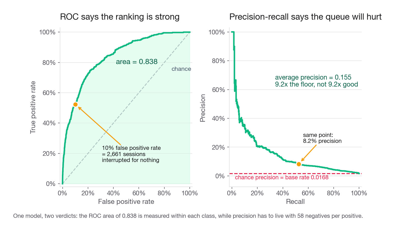
The ROC curve traces true positive rate against false positive rate as the threshold sweeps from one to zero. Both axes are normalized within a class, so the curve does not move when the ratio of positives to negatives changes. That is genuinely useful: the area under it, 0.838 here, is comparable across products with different base rates and across an undersampled run and a full one.
That same property is what makes it dangerous. A false positive rate of 10 percent sounds small. On 26,546 negatives it is 2,661 interrupted onboarding sessions.
from sklearn.metrics import roc_curve, roc_auc_score, average_precision_score

fpr, tpr, thr = roc_curve(y_te, p_hat)
pos, neg = int(y_te.sum()), int((y_te == 0).sum())
for target in [0.02, 0.05, 0.10, 0.20]:
    i = int(np.argmin(np.abs(fpr - target)))
    TP, FP = tpr[i] * pos, fpr[i] * neg
    print(round(fpr[i], 3), round(tpr[i], 3), round(thr[i], 4),
          int(TP), int(FP), round(TP / (TP + FP), 4))
print(round(roc_auc_score(y_te, p_hat), 4),
      round(average_precision_score(y_te, p_hat), 4))
0.020 0.269 0.1055 122 532 0.1865
0.050 0.394 0.0607 179 1322 0.1193
0.100 0.524 0.0369 238 2661 0.0821
0.200 0.725 0.0202 329 5310 0.0583
0.838 0.155| Point on the ROC curve | Bookings caught | Sessions interrupted for nothing | Precision |
|---|---|---|---|
| FPR 2 percent, TPR 27 percent | 121 | 532 | 18.7 percent |
| FPR 5 percent, TPR 39 percent | 179 | 1,322 | 11.9 percent |
| FPR 10 percent, TPR 52 percent | 237 | 2,661 | 8.2 percent |
| FPR 20 percent, TPR 73 percent | 329 | 5,310 | 5.8 percent |
The 10 percent row is a respectable-looking ROC point and eleven interruptions per booking in the real world. Nothing on the ROC axes reveals that, because neither axis knows there are 58 negatives for every positive.
Precision-recall: the curve whose floor moves
The precision-recall curve fixes that by putting precision, which mixes the two classes, on one axis. Precision is the share of your alerts that were right, and it degrades fast when negatives outnumber positives, exactly as an on-call rotation would.
The crucial reading habit: the baseline for average precision is not 0.5, it is the base rate. A coin flip achieves precision equal to the prevalence at every recall, so our floor is 0.0168 and our model's 0.155 is a lift of about 9.2 times over guessing. That is the honest one-line summary of this model's ranking ability.
| ROC / AUC | Precision-recall / average precision | |
|---|---|---|
| Axes | TPR against FPR | Precision against recall |
| Baseline for a useless model | 0.5, always | The base rate, 0.0168 here |
| Changes if you resample the classes | No | Yes, strongly |
| Reflects alert volume you must staff | No | Yes, directly |
| Good for comparing across products | Yes | Only at the same base rate |
| Good for choosing an operating point | Poor | Good |
| Sensitive to gains on the top 1 percent of scores | Weakly | Strongly |
Use both, and say why: ROC to compare model versions and to reason about ranking quality independent of prevalence, precision-recall to talk to a product manager about what the queue will feel like.
Interview tip: If you quote an average precision number, quote the base rate in the same breath. "AP of 0.155 against a 0.0168 floor" is a complete claim, "AP of 0.155" is not.
Fix one: move the threshold using an explicit cost matrix
Now the decision half. The default cut-off of 0.5 does have a justification behind it, just not one you want here. When the probabilities are calibrated and the two mistakes cost the same, 0.5 minimizes the expected number of misclassifications, and that holds at any prevalence. It is why 0.50 posted the best accuracy of any rule in the strategy table earlier, at a 1.68 percent base rate. So the problem is not that 0.5 is the wrong error-minimizer. The problem is that error count is the wrong objective when a miss costs 96 and a false alarm costs 3.20, a ratio of 30 to 1.
Write the four cells down first
Before any code, put numbers in four cells. Interviewers reward this because it forces the assumptions into the open where they can be argued with.
| Model says show | Model says skip | |
|---|---|---|
| Would have booked | Gain 96 in expected margin | Gain 0, forgo 96 |
| Would not have booked | Lose 3.20 in activation friction | 0 |
Two quantities fall out. The benefit of catching a positive, which is the difference between the two cells in the top row, is 96. The cost of a false alarm, the difference across the bottom row, is 3.20. Everything else in the matrix is a baseline you can subtract away.
The threshold formula, derived in three lines
For a session with predicted booking probability p, showing the modal has expected value 96p - 3.20(1 - p) and skipping it has expected value zero. Show it when the first exceeds the second:
96p - 3.20(1 - p) > 0
96p + 3.20p > 3.20
p > 3.20 / (96 + 3.20) = 0.0323
In general, with B the benefit of a caught positive and C the cost of a false alarm, the optimal cut-off is C / (B + C). Commit that to memory. It is the single most reusable formula in this topic and it takes ten seconds to derive at a whiteboard if you forget it.
Two sanity checks. If a false alarm costs nothing the threshold goes to zero and you act on everyone, which is correct. If missing a positive costs nothing it goes to one and you never act, also correct. And note what never appears in the formula: the base rate. Prevalence affects how many rows clear the bar, not where the bar sits.
Applying it
def value_at(scores, truth, t, benefit=96.0, cost=3.20):
    flag = scores >= t
    TP = int((flag & (truth.values == 1)).sum())
    FP = int((flag & (truth.values == 0)).sum())
    FN = int(truth.sum()) - TP
    return dict(t=t, TP=TP, FP=FP, FN=FN,
                precision=round(TP / max(TP + FP, 1), 4),
                recall=round(TP / int(truth.sum()), 4),
                value=round(benefit * TP - cost * FP, 1))

for t in [0.005, 0.010, 0.0168, 0.0323, 0.05, 0.08, 0.12, 0.20, 0.50]:
print(value_at(p_hat, y_te, t))| Cut-off | Bookings caught | False alarms | Precision | Recall | Value on 27,000 sessions |
|---|---|---|---|---|---|
| 0.005 | 428 | 14,841 | 2.8 percent | 94.3 percent | -6,403 |
| 0.010 | 384 | 9,772 | 3.8 percent | 84.6 percent | 5,594 |
| 0.0168 (base rate) | 343 | 6,337 | 5.1 percent | 75.6 percent | 12,650 |
| 0.0323 (from costs) | 255 | 3,117 | 7.6 percent | 56.2 percent | 14,506 |
| 0.05 | 198 | 1,773 | 10.1 percent | 43.6 percent | 13,334 |
| 0.08 | 159 | 877 | 15.4 percent | 35.0 percent | 12,458 |
| 0.12 | 106 | 410 | 20.5 percent | 23.3 percent | 8,864 |
| 0.20 | 54 | 118 | 31.4 percent | 11.9 percent | 4,806 |
| 0.50 (library default) | 2 | 0 | 100 percent | 0.4 percent | 192 |
The derived cut-off wins by a factor of 76 over the default. Per session that is 0.54, and at 11,000 first-day sessions a week it annualizes to roughly 314,000. All of it came from changing one number in a comparison operator: no new features, no new model, no retraining.
Three things here are worth saying out loud in an interview.
First, the value curve is flat near the top. Anything between about 0.025 and 0.05 lands within ten percent of the best value, so your cost estimates need only be roughly right and in the right order of magnitude.
Second, grid-searching the threshold that maximizes measured value on this same test set lands on 0.0257 with a value of 15,491. That looks better than the derived 0.0323 and it is a trap: you have fitted a parameter to your evaluation set, and a 7 percent edge is inside the noise generated by 454 positives. The derived threshold is a claim about the world and will hold next quarter. The tuned one is a fact about this sample.
Third, precision rises monotonically as you raise the bar and value does not. The peak sits where the marginal booking gained is worth exactly the marginal batch of interruptions it costs. Candidates who reflexively "maximize F1" are asserting that the two mistakes cost the same, which here is off by a factor of thirty.
The threshold is a function of costs, so stress test the costs
The right follow-up to "what threshold" is "how sensitive is that to your assumptions". Change the intervention and the whole operating point moves, with no model change at all.
| Scenario | Benefit of a booking | Cost of a false alarm | Cut-off | Share of sessions flagged | Precision | Recall |
|---|---|---|---|---|---|---|
| Inline banner, minimal friction | 96 | 0.85 | 0.0088 | 41.0 percent | 3.5 percent | 86.1 percent |
| Takeover modal (current) | 96 | 3.20 | 0.0323 | 12.5 percent | 7.6 percent | 56.2 percent |
| Full-screen interstitial | 96 | 7.40 | 0.0716 | 4.5 percent | 13.8 percent | 37.0 percent |
| Modal, but close rate halves | 48 | 3.20 | 0.0625 | 5.4 percent | 12.2 percent | 39.0 percent |
Make the interruption cheaper and you should show the modal to four in ten sessions. Make it more intrusive and fewer than one in twenty. Same scores, same ranking, wildly different product. This table is usually the most senior-sounding thing you can produce here, because it shows you treat the model as one input to a decision rather than as the decision.
When volume is capped, forget the threshold and take the top K
A threshold produces a variable alert volume, which is fine for a modal and disastrous for anything staffed by humans. If Larkfield caps how many onboarding sessions it is willing to interrupt in a period, the right object is not a probability cut-off but a rank cut-off: sort by score, take the top K, and let the implied threshold be whatever score sits at position K. The table below is computed over the whole 27,000-row test set, which is 2.4 weeks of traffic at 11,250 first-day sessions a week.
| Alert budget K (sessions shown) | Implied score cut-off | Bookings caught | Precision at K | Recall |
|---|---|---|---|---|
| 400 | 0.137 | 88 | 22.0 percent | 19.4 percent |
| 800 | 0.093 | 136 | 17.0 percent | 30.0 percent |
| 1,500 | 0.061 | 179 | 11.9 percent | 39.4 percent |
| 3,000 | 0.036 | 243 | 8.1 percent | 53.5 percent |
Precision at K is the metric an ops team can feel: at K equal to 800, roughly one in six of the sessions you flag ends in a booked call, and the other five absorb an interruption for nothing. Report precision at K rather than an area under a curve whenever a human queue is involved.
Be careful what K counts. It is modals shown, not calls booked. Those 800 modals produce 136 bookings across 2.4 weeks, about 57 calls a week, so a specialist team sized for 800 calls would sit idle. If specialist hours are the binding resource you have to invert through precision, and because precision is itself a function of K, that is a fixed point you solve for rather than a single division.
| Weekly specialist call capacity | Sessions to interrupt per week | Implied cut-off | Precision |
|---|---|---|---|
| 25 | 85 | 0.188 | 29.6 percent |
| 50 | 255 | 0.110 | 19.6 percent |
| 75 | 626 | 0.061 | 12.0 percent |
| 100 | 1,220 | 0.037 | 8.2 percent |
| 150 | 3,333 | 0.014 | 4.5 percent |
There is a hard ceiling here: showing the modal to all 11,250 sessions in a week yields only about 189 calls, so any staffing above that is slack and the cost-derived cut-off of 0.0323 governs instead. Note too that the 100-calls row implies 0.037, near enough to the derived 0.0323 that capacity and economics agree at that staffing level. Below it capacity binds, above it cost does.
Interview tip: Never answer "what threshold would you use" with a number. Answer with the formula and then ask for the two costs. If the interviewer refuses to give them, invent them out loud and mark them as assumptions.
Calibration: the cut-off is only as good as the probabilities
The threshold formula assumes p means something. If the model says 0.04 for a group of sessions and 9 percent of them book, a cut-off of 0.0323 is not implementing the rule you derived. Calibration is what makes the arithmetic legal. Check it by bucketing predictions and comparing the average prediction with the observed rate inside each bucket.
bins = [0, 0.005, 0.01, 0.02, 0.04, 0.08, 0.15, 1.0]
grp = pd.cut(p_hat, bins, include_lowest=True)
cal = (pd.DataFrame({"p": p_hat, "y": y_te.values})
         .groupby(grp, observed=True)
         .agg(n=("y", "size"), predicted=("p", "mean"), observed=("y", "mean")))
print(cal.round(4))| Score bucket | Sessions | Mean predicted | Observed rate |
|---|---|---|---|
| 0 to 0.005 | 11,731 | 0.0023 | 0.0022 |
| 0.005 to 0.01 | 5,113 | 0.0072 | 0.0086 |
| 0.01 to 0.02 | 4,462 | 0.0142 | 0.0121 |
| 0.02 to 0.04 | 3,069 | 0.0278 | 0.0323 |
| 0.04 to 0.08 | 1,589 | 0.0550 | 0.0453 |
| 0.08 to 0.15 | 708 | 0.1065 | 0.1102 |
| above 0.15 | 328 | 0.2264 | 0.2470 |
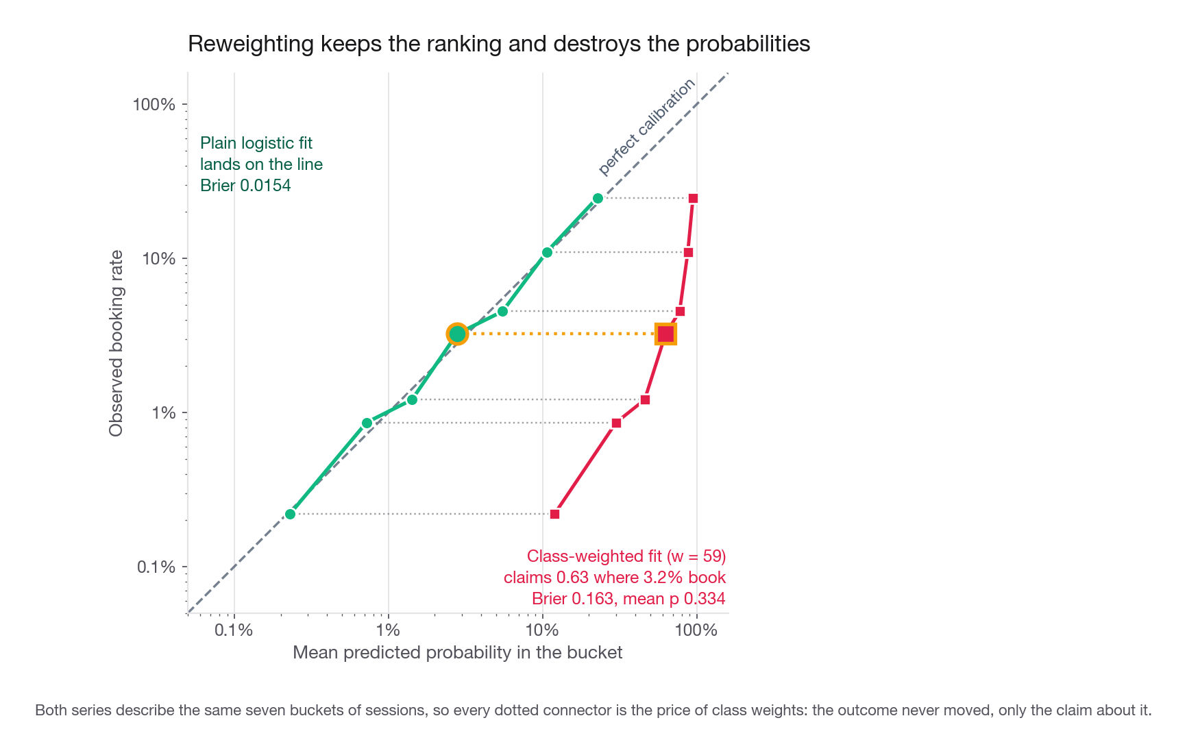
Predicted and observed track to within a few thousandths in every bucket. Logistic regression fitted on full data with log loss tends to come out this way, because log loss is a proper scoring rule and the intercept absorbs the prevalence. Summarize with the Brier score, mean squared error on probabilities: 0.0154 here.
Three model families routinely fail this check, and knowing which is a cheap way to sound experienced:
Random forests average votes across trees, which pulls extreme predictions toward the middle. They rarely emit probabilities near zero or one even when they should.
Boosted trees run too long do the opposite: they push scores toward the extremes and become overconfident.
Anything trained on reweighted or resampled data is miscalibrated by construction, which is the subject of the next section and is by far the most common cause in practice.
The fix is a monotone recalibration fitted on held-out data: Platt scaling, a one-variable logistic regression on the raw score, or isotonic regression, which is more flexible and needs more data. Both are monotone, so neither changes the ranking and ROC AUC is untouched. What changes is that your derived threshold becomes meaningful again.
Interview tip: Say "AUC is invariant to any monotone transform of the score, so recalibration cannot change it, but it can completely change whether my threshold is right." That single sentence separates candidates who have shipped a model from candidates who have read about one.
Fix two: reweight the classes during training
Threshold tuning is the first tool because it is cheap, reversible, and leaves the model untouched. It has exactly one failure mode, and it is total.
When the threshold has nothing to work with
Suppose the learner never finds a split worth making. At a base rate of 1.68 percent the Gini impurity at the root is about 0.033, so almost every candidate split improves purity by a rounding error. Set a modest minimum improvement and the tree refuses to split at all.
from sklearn.tree import DecisionTreeClassifier

flat = DecisionTreeClassifier(min_impurity_decrease=0.001, random_state=7)
flat.fit(X_tr, y_tr)
p_flat = flat.predict_proba(X_te)[:, 1]
print(flat.get_n_leaves(), len(np.unique(p_flat)), round(float(p_flat[0]), 5))
1 1 0.01681One leaf, one distinct predicted probability, and that probability is the training prevalence. There is no ranking to threshold: every cut-off above 0.0168 flags nobody, every cut-off at or below it flags everybody, and a threshold sweep produces a table with two rows in it.
This is not contrived. It happens whenever an impurity criterion, a regularization penalty, or an early-stopping rule calibrated for balanced data gets pointed at a 1-in-60 label. The learner correctly concludes that the cheapest way to reduce loss is to do nothing.
What reweighting actually does
Give each minority row a weight of w and the loss behaves as though you had w copies of it. In a tree the impurity calculation counts a positive as w observations, so root impurity climbs and splits that isolate positives start clearing the improvement bar. In logistic regression each positive contributes w times as much gradient, so the fit can no longer ignore them.
The mental model that survives follow-ups: reweighting adds no information, it changes the exchange rate the optimizer uses between the two kinds of mistake. It is the training-time version of the decision you were already making at threshold time.
Watch the same tree wake up when only the weights change.
weighted = DecisionTreeClassifier(min_impurity_decrease=0.001,
                                  class_weight={0: 1, 1: 59}, random_state=7)
weighted.fit(X_tr, y_tr)
print(weighted.get_n_leaves(),
      round(roc_auc_score(y_te, weighted.predict_proba(X_te)[:, 1]), 4))
26 0.7945Twenty-six leaves and an AUC of 0.79, from a model that was a constant a moment ago. The weight of 59 is not magic: it is the ratio of negatives to positives in training, which is what class_weight="balanced" computes for you.
The weight sweep, and what it does and does not move
Now the part most candidates get wrong. Sweep the minority weight on the logistic model and watch four quantities.
rows = []
for w in [1, 5, 10, 20, 40, 59, 100]:
    m = LogisticRegression(max_iter=3000, class_weight={0: 1, 1: w}).fit(X_tr, y_tr)
    s = m.predict_proba(X_te)[:, 1]
    hard = (s >= 0.5)
    TP = int((hard & (y_te.values == 1)).sum())
    FP = int((hard & (y_te.values == 0)).sum())
    rows.append([w, round(roc_auc_score(y_te, s), 4),
                 round(float(np.mean((s - y_te.values) ** 2)), 5),
                 round(float(s.mean()), 4), TP, FP])
print(pd.DataFrame(rows, columns=["w", "auc", "brier", "mean_p", "TP", "FP"]))| Minority weight | ROC AUC | Brier score | Mean predicted probability | Recall at 0.5 | Precision at 0.5 | Accuracy at 0.5 |
|---|---|---|---|---|---|---|
| 1 | 0.8377 | 0.0154 | 0.0167 | 0.4 percent | 100 percent | 98.3 percent |
| 5 | 0.8379 | 0.0221 | 0.0668 | 15.6 percent | 27.2 percent | 97.9 percent |
| 10 | 0.8379 | 0.0363 | 0.1129 | 30.0 percent | 16.7 percent | 96.3 percent |
| 20 | 0.8378 | 0.0663 | 0.1808 | 44.9 percent | 9.9 percent | 92.2 percent |
| 40 | 0.8377 | 0.1202 | 0.2726 | 67.2 percent | 6.6 percent | 83.5 percent |
| 59 (balanced) | 0.8377 | 0.1632 | 0.3337 | 76.0 percent | 5.1 percent | 75.9 percent |
| 100 | 0.8376 | 0.2374 | 0.4252 | 84.8 percent | 3.8 percent | 63.2 percent |
Stare at the second column. ROC AUC moves in the fourth decimal place across a hundredfold change in weight. The Spearman correlation between the unweighted and the balanced scores is 0.9994. Reweighting a well-specified model barely changes the ranking. What it changes is where the default cut-off happens to land on that ranking, plus, catastrophically, the calibration: the Brier score degrades by a factor of eleven and the average predicted probability drifts from 0.0167, which matched the true prevalence almost exactly, to 0.3337, which is off by a factor of twenty.
That is the single most useful sentence in this lesson. Reweighting is, for a model that was already fitting fine, an expensive and probability-destroying way to move the threshold.
| Quantity | Changes when you reweight? | Why |
|---|---|---|
| Ranking of records by score | Barely, in a well-specified model | The relative ordering is driven by the features, not the loss weights |
| ROC AUC | Barely | It depends only on the ranking |
| Average precision | Barely | Same reason, though it is noisier at low prevalence |
| Predicted probabilities | Drastically | The model now targets a synthetic prior, not the real one |
| Brier score and reliability | Drastically, for the worse | Direct consequence of the shifted prior |
| Meaning of the 0.5 cut-off | Completely | Which is the only reason it appears to help |
| Ability to fit at all when the learner degenerates | Yes, decisively | Higher root impurity makes splits worth taking |
| Variance of the fit | Increases | Effective sample size drops toward the minority count |
Reweighting without a re-derived threshold is a downgrade
Prove it on the same test set. Take the balanced model and score it at the default cut-off, which is what most people do.
| Configuration | Bookings caught | False alarms | Value on 27,000 sessions |
|---|---|---|---|
| Plain model, cut-off 0.50 | 2 | 0 | 192 |
| Balanced weights, cut-off 0.50 | 345 | 6,408 | 12,614 |
| Plain model, cut-off 0.0323 from costs | 255 | 3,117 | 14,506 |
| Balanced weights, cut-off re-derived to 0.663 | 251 | 3,080 | 14,240 |
| Undersampled 1-to-1, probabilities corrected, cut-off 0.0323 | 257 | 3,102 | 14,746 |
Balanced weights at the default cut-off is a big improvement over the default cut-off alone, which is why it feels like it works. It is still 13 percent worse than leaving the model alone and choosing the threshold properly. And once you re-derive the threshold on the reweighted scale, all four sensible configurations collapse into a band from 14,240 to 14,746, which is the noise floor for 454 positives. The rebalancing was never the lever. The threshold was.
Getting your probabilities back
If you did reweight, or undersample, you can undo the prior shift analytically. When the negative class is downsampled by a factor r, or the positive class is upweighted by w, the reported probability q maps back to the true-prior probability with:
def restore_prior(q, factor):
    return q / (q + (1.0 - q) * factor)

print(round(float(restore_prior(np.array([0.6632]), 59.0)[0]), 4))0.0323Applying that to the balanced model brings the mean prediction back to 0.0165 against a true 0.0168, and the Brier score back to 0.0154 from 0.163, with the AUC unmoved at 0.8377. Equivalently, run it in the other direction to find the cut-off on the reweighted scale that corresponds to your derived one: a true-prior threshold of 0.0323 maps to 0.663 when the minority weight is 59, which is why "balanced weights plus the 0.5 default" ends up too aggressive.
Resampling, reweighting, or thresholding: pick with reasons
Undersampling the majority class, oversampling the minority, and reweighting are close cousins. Duplicating a minority row w times and giving it weight w produce the same expected loss surface. Undersampling is different in one important way: it throws data away, which is a real cost when the majority class carries most of the information about where the boundary is not, and a real benefit when you have 40 million negatives and a training budget.
Two operational rules about resampling that interviewers probe for.
Resample only the training fold, never the evaluation fold. If you rebalance before splitting, near-duplicate minority rows land on both sides and your holdout precision becomes fiction. With SMOTE the leak is worse, because a synthetic point can be a near-interpolation of a test row.
Never resample the thing you are measuring. Precision, average precision, and expected value are all functions of the class ratio. Compute them on a test set that has the production prevalence, or every number you report is describing a world that does not exist.
On synthetic minority oversampling specifically: it interpolates between a minority point and its neighbours, which assumes the region between two positives is also positive. For continuous, locally smooth features that is often reasonable. For a one-hot acquisition channel it produces a session that is 0.4 webinar and 0.6 partner, which is not a session. If your feature matrix is mostly dummies, reach for weights instead.
Interview tip: Asked "would you use SMOTE", the strong answer is "probably not first", followed by the leakage rule and the one-hot objection. Enthusiasm for SMOTE without those caveats is a common junior tell.
Common traps
Reporting accuracy, or optimizing it, on a skewed label. The fix is to report recall at a fixed alert budget alongside precision at that budget, and to lead with expected value once you have costs.
Treating 0.5 as meaningful. It is a library default that encodes exactly one assumption: that the two mistakes cost the same. It does not assume balanced classes. With calibrated probabilities 0.5 minimizes error count at any prevalence, which is why it wins on accuracy at Larkfield and still creates almost no value. Derive the cut-off from
C / (B + C)and say the two costs out loud.Tuning the threshold to maximize measured value on the test set. You will beat the derived threshold on that sample and lose next quarter. Derive it, then use the test set only to confirm the value curve is flat around your choice.
Rebalancing and then keeping the default cut-off. This is really an undeclared threshold change with the side effect of ruining your probabilities. It cost 13 percent of the available value in the Larkfield table.
Quoting probabilities from a reweighted or undersampled model. The mean prediction drifted from 0.0167 to 0.3337 in our sweep. Either correct with
q / (q + (1 - q) * factor)or recalibrate on a held-out fold at production prevalence.Resampling before the train-test split. Duplicated or interpolated minority rows straddle the split and inflate every holdout metric. Split first, resample inside the training fold only.
Expecting reweighting to improve ranking. Across weights from 1 to 100, our AUC moved by 0.0003. If the ranking is bad, weights will not fix it; better features or a better label will.
Maximizing F1 by reflex. F1 asserts that a missed positive and a false alarm cost the same. At Larkfield the ratio is 30 to 1, so F1 quietly picks the wrong operating point.
Ignoring capacity. A probability threshold produces variable volume. If the alert budget is fixed, or a human touches each alert, rank and take the top K, and report precision at K.
Forgetting that the label is only valid where the treatment was applied. Larkfield's label exists because the modal was shown to everyone for eight weeks. Once you start targeting, the training distribution drifts away from the population you score, and you need a small random holdout that keeps seeing the modal to refresh the label.
Confusing "will book if shown" with "books because it was shown". Our model predicts the former, which is the right object for a show-or-skip decision under a fixed treatment. If the question is who is changed by the modal, that is an uplift problem and a different label entirely.
Quick self-check
Answer each of these aloud, in under a minute, before you look anything up.
Your model reaches 99.1 percent accuracy on a label with a 1.2 percent positive rate. What is the first number you ask for, and what would make the accuracy figure genuinely impressive?
Catching a fraudulent refund saves 210. Wrongly holding a legitimate refund costs 14 in support time and goodwill. What cut-off do you use, and what happens to it if the support team gets cheaper?
You retrain with
class_weight="balanced"and ROC AUC is unchanged to three decimals, but recall at the default cut-off jumps from 3 percent to 71 percent. Explain in two sentences what actually happened.A colleague reports average precision of 0.21 and calls the model strong. What single number do you need before you can agree or disagree?
Your tree produces exactly one distinct predicted probability across the whole holdout. Name the value it will be equal to, explain why threshold tuning cannot help, and say what you would change first.
You undersample negatives 40 to 1 for training speed. A product manager asks what share of flagged accounts will actually convert. What do you have to do to the model output before you can answer, and what would the raw number have told them?